Put-Call Parity and Arbitrage Strategies

Introduction

In this chapter, we will discuss the option's payoff if you long or short the options. Then we discuss the put-call parity which is a relationship between the price of a European call option, the price of a European put option, and the underlying stock price. In addition, an application of put-call parity in arbitrage trading strategies was demonstrated.

Option Payoff

Consider Google(NASDAQ: GOOG) is trading at $910 now and you are bullish on this stock and expect it to rise over the next three months. The minimum capital requirement to buy 100 shares of GOOG is $90000 but you only have limited capital for stock investors. You could buy 1 call option contract written on GOOG which expires after three months with a $900 strike price. If GOOG rises to $950 in three months, you can get  ($950 - $900) * 100 = $5000 by paying just a small amount of premium instead of a full cost of shares. Even if the share price of GOOG falls below $900, you lose only the premium. This is one of the biggest benefits of trading options and is also called the financial leverage. Without borrowing the capital, you can control a larger number of shares by investing in options other than purchasing the shares themselves.

From the above example, the investor will buy a European call if he has a bullish view on the market and believes the underlying stock price will be above the strike price at the expiry date. He will make money when the underlying price goes up and lose when it goes down. The payoff of a call option at T is

$$Call_{payoff}=\max(S_T-K, 0)$$

On the other hand, an investor will buy a European put if he is bearish about the market and believes that the underlying stock price will be below the strike at the expiry date. He will make money when the underlying price goes down and lose when it goes up. The European put payoff at T is

$$Put_{payoff}=\max(K-S_T, 0)$$

Where $S_T$ is the price of underlying assets at maturity. K is the strike price.

We use the GOOG option contract to show the call and put option payoff. The current share price of GOOG is $945 at 07/12/2017.

Contract Name	Type	Expire Date	Strike	Premium
GOOG 170714C00940000	Call	07/14/2017	$940	$7.5
GOOG 170714P00960000	Put	07/14/2017	$960	$19.5

If you long these two options, the payoff at expiration date would be as follows

import matplotlib.pyplot as plt
%matplotlib inline
price = np.arange(900,1000,1)
strike = 940
premium = 7.5
payoff = [max(-premium, i - strike-premium) for i in price]
plt.plot(price, payoff)
plt.xlabel('Price at T S_T ($)')
plt.ylabel('payoff')
plt.title('Call option Payoff at Expiry')
plt.grid(True)
price = np.arange(900,1000,1)
strike = 960
premium = 19.5
payoff = [max(-premium, strike - i -premium) for i in price]
plt.plot(price, payoff)
plt.xlabel('Price at T S_T ($)')
plt.ylabel('payoff')
plt.title('Put option Payoff at Expiry')
plt.grid(True)

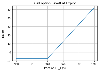
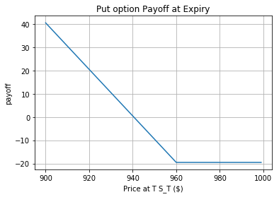
The above payoff diagrams illustrate the cash payoff on an option at the expiration date. For a call option, the net payoff is negative if the price of the underlying asset is less than the strike price(The negative payoff comes from the premium). If the underlying price exceeds the strike price, the gross payoff is the price of the underlying asset minus the strike price and the premium. For a put option, the net payoff is positive if the underlying price is less than the strike price. If the price of the underlying asset exceeds the strike price, the gross payoff is negative because you pay the premium for purchasing the contracts.

Put-Call Parity

Put-Call parity describes the relationship between the price of a European put and a call options with the identical strike price K, expiry T and their underlying stock's price. Next, we will demonstrate how to derive the put-call parity according to John Hull's book.

We consider two portfolios as follows,

Portfolio A: buy one European call option (underlying non-dividend-paying stock S, strike K, expiring at T) plus a zero-coupon bond which pays K at T

Portfolio B: sell one European put option (underlying non-dividend-paying stock S, strike K, expiring at T) plus one share of underlying stock S

Payoff	$S_t > K$	$S_t < K$
Portfolio A	$S_t - K+K=S_t$	$0+K=K$
Portfolio B	$0+S_t =S_t$	$K-S_t+S_t=K$

From the above table we can see that in all states, Portfolio A has the same payoff at the options' expiration date as Portfolio B. Thus the present value of two portfolios must be the same. Otherwise, an investor can make risk-free profits by purchasing the undervalued portfolio and selling the overvalued portfolio and holding the position to maturity. Then we have the price equality(suppose the present price of stock S is $S_0$ )

$$P_{call}+Ke^{-rT}=P_{put}+S_0$$

If the dividend is paid during the option holding period, the shareholder of the stock would receive that additional amount, but the option owner would not. For a dividend-paying stock, the put-call parity relationship is (D is the present value of dividends):

$$P_{call}+D+Ke^{-rT}=P_{put}+S_0$$

Synthetic Positions

Through the put-call parity, we can find that there is a synthetic equivalent for all of the basic positions in underlying assets and its corresponding options. In other words, the risk profile (the possible profit or loss) of any position can be exactly duplicated with a complex combination of the other basic positions. These equivalents are synthetic underlying and synthetic options.

The rule for creating synthetics is that the strike price and expiration date, of the calls and puts, must be identical. For creating synthetics, with both the underlying stock and its options, the number of shares of stock must equal the number of shares represented by the options.

There are many arbitrage strategies based on the idea of the synthetic position. Here we demonstrate two of the most common strategies: the conversion and the reversal.

Strategy	Content
Conversion	Synthetic Short Position: short call + long put The actual stock position: long the underlying stocks
Reversal	Synthetic Long Position: long call + short put The actual stock position: short the underlying stocks

Traders use conversions when options are overpriced relative to the underlying stock and use reversals when options are relatively underpriced.

Summary

In this chapter, we derived an important relationship between the prices of European put and call options that have the same strike price and time to maturity by constructing two portfolios. Then we described the synthetic positions, a common concept which is always used in arbitrage trading strategies. Finally two simple arbitrage strategies conversion and reversal are demonstrated on QC platform to help you get a better understanding of how to implement algorithms with simple option mechanism.

Next chapter we will dig into the famous option pricing model - Black–Scholes–Merton Model and discuss how to apply BSM in European options pricing.

---

---

---