Stochastic Processes and Monte Carlo Method

Introduction

Last few chapters we introduced the basic principles and mechanism of options trading. We already knew what an option contract is and the basic relationship between call and put options' price. But how do these contracts traded in the exchange are being priced and where does the option premium come from? In the next few chapters, we will discuss the pricing of options.

Brownian motion

In order to value the derivatives like options, the most significant part is to find a model to represent the underlying stock price so that we can price the options based on the underlying price. We usually use the stochastic process to model the security price.

First, you need to know what the stochastic process is. We say any variable that changes over time in an uncertain way follows a stochastic process. The price of a certain stock at a future time t is unknown at the present so it is a random variable $S_t$. Then we can think of the movement path of the stock price is a stochastic process since $S_t$ is a random variable at each time t in the future.

Markov process is a special case of the stochastic process. It means that only the current value of a random variable is relevant for future prediction. In general, we usually assume that the stock price follows a Markov stochastic process, which means only the current stock price is relevant for predicting the future price, it is not correlated with the past price.

Brownian motion is a particular type of Markov stochastic process or we can think of it as a family of random variables $\left\{W_t\mid t\geq0\right\}$ indexed by time t. The one-dimensional Brownian motion is called the Wiener Process. (Brownian motion is n-dimensional Wiener processes which mean each dimension is just a standard Wiener process). It has the following properties:

• $W_0=0$
• For $t\geq0$ and $\Delta t\geq0$, the increment $W_{t+\Delta t}-W_t$ is normally distributed with mean 0 and standard deviation $\sqrt{\Delta t}$ .
• For any partitions $0\leq t_1<t_2<\cdot\cdot\cdot <t_n$, the increments $W_{t_1}- W_{t_0},W_{t_2}-W_{t_1},\cdot\cdot\cdot, W_{t_n}-W_{t_{n-1}}$ are independent random variables.
• With probability 1, the function W(t) is continuous at t.

Intuitively understanding of the definition, Wiener process has independent and normally distributed increments and has continuous sample path.

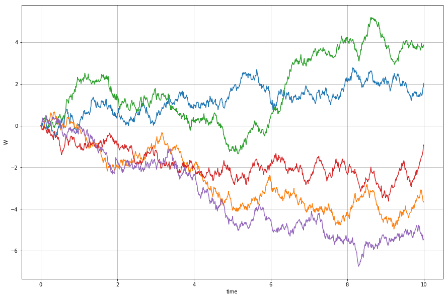
Next, we simulate the Wiener process and plot the paths attempting to gain an intuitive understanding of a stochastic process. Each path is an independent Wiener process.

import numpy as np
import matplotlib.pyplot as plt
%matplotlib inline
def wiener_process(T, N):
    """
    T: total time
    N: The total number of steps
    """
    W0 = [0]
    dt = T/float(N)
    # simulate the increments by normal random variable generator
    increments = np.random.normal(0, 1*np.sqrt(dt), N)
    W = W0 + list(np.cumsum(increments))
    return W

N = 1000
T = 10
dt = T / float(N)
t = np.linspace(0.0, N*dt, N+1)
plt.figure(figsize=(15,10))
for i in range(5):
    W = wiener_process(T, N)
    plt.plot(t, W)
    plt.xlabel('time')
    plt.ylabel('W')
    plt.grid(True)

In ordinary calculus, $\text{d}x=a\ \text{d}t$ is used to indicate that $\Delta x=a\Delta t$ as $\Delta t\rightarrow0$. We use the similar notation here. The mean change per unit time for a stochastic process is known as the drift rate and the variance per unit time is known as the variance rate. We can write the derivative of Wiener process over time t in this form: $dW_t$. A standard Wiener process has a drift rate (i.e. average change per unit time) of 0 and a variance rate of 1 per unit time. If we extend the concept of Wiener process to a generalized Wiener process in the form: $\text d\ x_t=a\ \text d t+b\ \text dW_t$. The drift rate and the variance rate can be set equal to any chosen constant. If we write it as approximate discrete form as

$$\Delta x=x_{t+\Delta t}-x_t=a\Delta t+b\epsilon\sqrt{\Delta t}$$

Where ε follows the standard normal distribution N(0,1). Thus $\Delta x$ has normal distribution with the mean being $a\Delta t$, variance being $b^2\Delta t$. And because $\Delta t$ is independent, from time 0 to time T, the change in the value of x is just the sum of $\Delta x$ in each small time interval. It means that the change in the value of x follows the normal distribution $N(aT,b^2T)$.

Modeling Stock Price as a Stochastic Process

Then we go back to the stock price. If we use the generalized Wiener process to model the stock price, for example, the share price of a stock is $30 now, then the percentage change in price from now to say the end of this year is normally distributed with constant mean and variance. But there is a problem that for normal distribution assumption of return, there is the possibility that the stock price will be negative this is unrealistic for stock prices. For example, this percentage change could be -1.1, which means the stock price at the end of the year is -$3.

On the other hand, if the spot price is small for a stock, then it tends to have small increments in price over a given time interval, on the contrary, stocks with high prices tend to have much larger increments in price on the same interval. But Wiener process has a variance which depends on just the time interval but not on the price itself. Thus it is not appropriate to assume that a stock price follows a generalized Wiener process with constant drift rate and variance rate.

In order to characterize the dynamics of a stock price process and fix this problem, we model the proportional increase in the stock price by using the stochastic differential equation (SDE):

$$\text dS_t=\mu S_t\ \text d t+\sigma S_t\ \text dW_t \cdot\cdot\cdot\cdot\cdot\cdot(1)$$

Where $dS_t$ is the change in the stock price over a short time period from $t$ to $t+\Delta t$. $μ$ is the drift term and can be deemed as the annual expected level of the stock return, $σ$ is the annual volatility of the stock. Here $dS_t$ at different time $t$ are independent, which means today's price change is independent with tomorrows change. $W_t$ is a standard Wiener process (1) we discussed above.

Now in the above equation, the drift and variance rate of stock price $S$ is not only correlated with time $t$ but also a function of both $S$ itself and time $t$.

The discrete approximation form of (1) is

$$\Delta S=\mu S\Delta t+\sigma S\epsilon\sqrt{\Delta t}$$

We can also derive the process that $\ln(S_t)$ follows (here we just give the result, but the derivation uses the Ito Lemma):

$$\begin{equation} \begin{aligned} \text d\ \ln(S_t) & = \left(\mu-\frac{\sigma^2}{2}\right) \ \text d t \\ & + \sigma \ \text dW_t \cdot\cdot\cdot\cdot\cdot\cdot (2) \end{aligned} \end{equation}$$

Here $\ln(S_t)$ follows a generalized Wiener process as which has constant drift rate and variance rate. That means the change in $\ln(S_t)$ during time interval $\Delta t$ is normally distributed. This is the lognormal property of stock prices.

$$\ln(S_{t+\Delta t})-\ln(S_t)\sim N\left[\left(\mu-\frac{\sigma^2}{2}\right)\Delta t,\sigma^2\Delta t\right]$$

$$\ln(S_{t+\Delta t})\sim N\left[\ln{S_t}+\left(\mu-\frac{\sigma^2}{2}\right)\Delta t,\sigma^2\Delta t\right]$$

Now the logarithm stock price follows the normal distribution. We write (2) into discrete approximation form as:

$$ln(S_{t+\Delta t})-\ln(S_{t})=\left(\mu-\frac{\sigma^2}{2}\right)\ \Delta t+\sigma \epsilon\sqrt{\Delta t}$$

Equivalently

$$S_{t+\Delta t}=S_{t}\exp\left[\left(\mu-\frac{\sigma^2}{2}\right)\ \Delta t+\sigma \epsilon\sqrt{\Delta t}\right]\cdot\cdot\cdot\cdot\cdot\cdot (3)$$

If we change t to 0 and change $\Delta t$ to T, we get

$$S_{T}=S_{0}\exp\left[\left(\mu-\frac{\sigma^2}{2}\right)\ T+\sigma \epsilon\sqrt{T}\right]$$

According to the above equation, we know the stock price at time $T$ should always be greater than 0 and the problem of having a negative price is fixed. Thus we say the stock price $S$ is a Geometric Brownian motion because the logarithm of $S$ follows a Brownian motion.

Monte Carlo Simulation of Stock Price

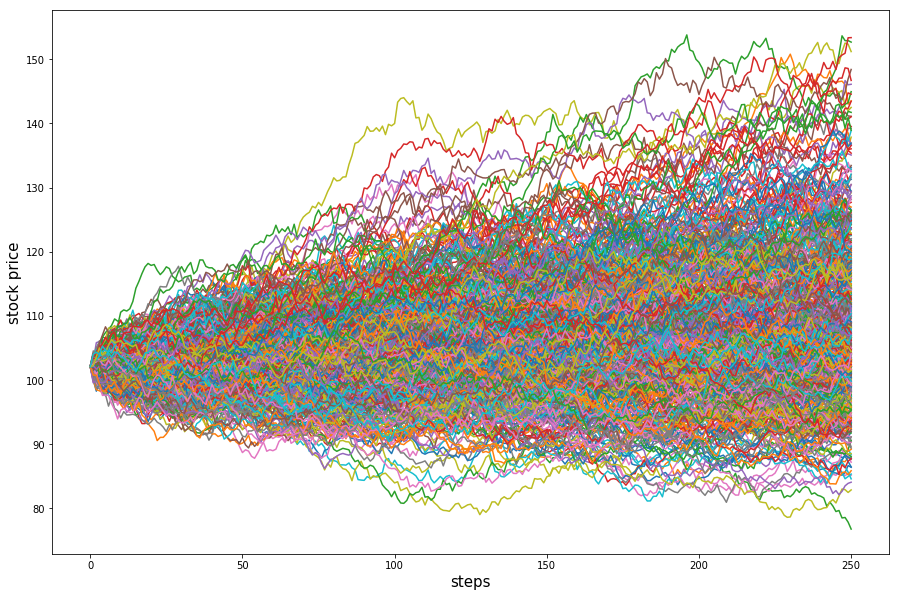
We apply this technique to model stock prices in order to look at the potential evolution of stock prices over time and then demonstrate how to price European options. Here we use Google as an example. Suppose today is 07/31/2017 and that the share price of GOOG is $930.5. We use the historical close price from 01/2015 to 07/2017 to compute the historical annual return and volatility as the $\mu$ and $\sigma$ parameters. (Note, we do not need to concern with the detailed determinants of $\mu$ because the value of options written on a stock is, in general, is independent of $\mu$. In contrast, the stock price volatility $\sigma$ is of crucial importance to the determination of the value of options). Consider GOOG that pays no-dividends, has an expected return 39.64% per annum with continuous compounding and a volatility of 23.44% per annum. Observe today’s price $903.5 per share and with $∆t$ = 0.001 yr. Then we apply Monte Carlo to simulate 500 price paths in the next three months.

from datetime import datetime 
qb = QuantBook()
goog = qb.AddEquity("GOOG").Symbol
close = qb.History(goog, datetime(2015,1,1), datetime(2017,8,1), Resolution.Daily).close

annual_return = (close[-1]/close[1])** (365.0/len(close)) - 1
annual_vol = (close/close.shift(1)-1)[1:].std()*np.sqrt(252)
mu = annual_return # 0.39856
sigma = annual_vol # 0.2343
s0 = close[-1]     # 43.92
T = 3.0/12
delta_t = 0.001
num_reps = 500
steps = T/delta_t
plt.figure(figsize=(15,10))
for j in range(num_reps):
    price_path = [s0]
    st = s0
    for i in range(int(steps)):
        st = st*e**((mu-0.5*sigma**2)*delta_t + sigma*np.sqrt(delta_t)*np.random.normal(0, 1))
        price_path.append(st)
    plt.plot(price_path)
plt.ylabel('stock price',fontsize=15)
plt.xlabel('steps',fontsize=15)

Monte Carlo Simulation of European Options

Monte Carlo simulation is a commonly used method for derivatives pricing where the payoff depends on the history price of the underlying asset.

The essence of using Monte Carlo method to price the option is to simulate the possible paths for stock prices then we can get all the possible value of stock price at expiration.

• First, we need to divide the maturity T of options into N small time intervals, the length of each time interval is $\Delta t$, N is the number of steps
• Sample the possible random paths for the stock price according to equation (3) and get the stock price $S_T$at maturity T.
• Calculate the payoff of options according to the $S_T$
• Discount the payoff at the risk-free rate to get one estimate of options' price
• Repeat the step 1 to 4 for a reasonable number of times and get many estimates of options price and then the average of these price estimates is the final options price.

In option pricing, Monte Carlo simulations use the risk-neutral valuation result. More specifically, sample the paths to obtain the expected payoff in a risk-neutral world (The expected annual return rate and the risk-free annual rate should be the same in order to get the correct estimation of the option) and then discount this payoff at the risk-neutral rate.

def mc_euro_options(option_type,s0,strike,maturity,r,sigma,num_reps):
    payoff_sum = 0
    for j in range(num_reps):
        st = s0
        st = st*e**((r-0.5*sigma**2)*maturity + sigma*np.sqrt(maturity)*np.random.normal(0, 1))
        if option_type == 'c':
            payoff = max(0,st-strike)
        elif option_type == 'p':
            payoff = max(0,strike-st)
        payoff_sum += payoff
    premium = (payoff_sum/num_reps)*e**(-r*maturity)
    return premium
mc_euro_options('c',927.96,785,100.0/252,0.01,0.23,500)

Suppose the risk-free rate is 1%. A European call option with strike price being $785 and expires in 100 days, the spot price is $927, the premium by using Monte Carlo method is $149.

Summary

In this chapter, we modeled stock price with the stochastic process. The stochastic process usually assumed for a stock price is geometric Brownian motion.The Black–Scholes–Merton model, which we cover in the next chapter, is based on the geometric Brownian motion assumption. Under this process, the logarithm of stock return in a small period of time is normally distributed and the returns in two nonoverlapping periods are independent.

In the second part of the tutorial, we applied Monte Carlo method to simulate the stock price in order to gain an intuitive understanding of the stochastic process followed by stock price. Then we discussed how to use Monte Carlo method to price the options based on the underlying prices paths.

---

---

---