Introduction
The change of volatility can have a significant impact on the performance of options trading. In addition to the Vega we explained in Greeks letter chapter, this part of the volatility tutorial will discuss the concept of volatility, specifically, we discuss realized and implied volatility, their meanings, measurements, uses, and limitations.
Historical Volatility
1. Definition
It is a measurement of how much the price of the asset has changed on average during the certain period of time. In common, volatility is said to be the standard deviation of the return of assets price.
2. Calculation
Next we discuss how to estimate the historical volatility of the option empirically.
Where (n+1) is the number of observations, is the stock price at end of it time interval
The standard deviation of the is given by
where is the mean of
If we assume there are n trading days per year. Then the estimate of historical volatility per annum is
import pandas as pd
from numpy import sqrt,mean,log,diff
from datetime import datetime
qb = QuantBook()

# use the daily data of Google(NASDAQ: GOOG) from 01/2016 to 08/2016
goog = qb.AddEquity("GOOG").Symbol
close = qb.History(goog, datetime(2016,1,1), datetime(2016,9,1), Resolution.Daily).close
r = diff(log(close))
r_mean = mean(r)
diff_square = [(r[i]-r_mean)**2 for i in range(0,len(r))]
sigma = sqrt(sum(diff_square)*(1.0/(len(r)-1)))
vol = sigma*sqrt(252)
An asset has a historical volatility based on its past performance as described above, investors can gain insight on the fluctuations of the underlying price during the past period of time. But it does not tell us anything about the volatility in the market now and in the future. So here we introduce the implied volatility.
Implied Volatility
In contrast to historical volatility, the implied volatility looks ahead. It is often interpreted as the market’s expectation for the future volatility of a stock and is implied by the price of the stock’s options. Here implied volatility means it is not observable in the market but can be derived from the price of an option.
1. Definition
We use volatility as an input parameter in option pricing model. If we take a look at the BSM pricing, the theoretical price or the fair value of an option is P, where P is a function of historical volatility σ, stock price S, strike price K, risk-free rate r and the time to expiration T. That is . But the market price of options is not always the same with the theoretical price. Now in contrast, if we are given the market’s prices of calls and puts written on some asset and also the value of S, K, r, T. For each asset we can solve a new volatility that corresponds to the price of each option – the implied volatility. Then the implied volatility is .
2. Calculation
Here we use the bisection method to solve the BSM pricing equation and find the root which is the implied volatility. We use Yahoo Finance Python API to get the real time option data.
import scipy.stats as stats

def bsm_price(option_type, sigma, s, k, r, T, q):
    # calculate the bsm price of European call and put options
    d1 = (np.log(s / k) + (r - q + sigma ** 2 * 0.5) * T) / (sigma * np.sqrt(T))
    d2 = d1 - sigma * np.sqrt(T)
    if option_type == 'c':
        return np.exp(-r*T) * (s * np.exp((r - q)*T) * stats.norm.cdf(d1) - k *  stats.norm.cdf(d2))
    if option_type == 'p':
        return np.exp(-r*T) * (k * stats.norm.cdf(-d2) - s * np.exp((r - q)*T) *  stats.norm.cdf(-d1))
    raise Exception(f'No such option type: {option_type}')

def implied_vol(option_type, option_price, s, k, r, T, q):
    # apply bisection method to get the implied volatility by solving the BSM function
    precision = 0.00001
    upper_vol = 500.0
    max_vol = 500.0
    min_vol = 0.0001
    lower_vol = 0.0001
    iteration = 50

    while iteration > 0:
        iteration -= 1
        mid_vol = (upper_vol + lower_vol)/2
        price = bsm_price(option_type, mid_vol, s, k, r, T, q)

        if option_type == 'c':
            lower_price = bsm_price(option_type, lower_vol, s, k, r, T, q)
            if (lower_price - option_price) * (price - option_price) > 0:
                lower_vol = mid_vol
            else:
                upper_vol = mid_vol
            if mid_vol > max_vol - 5 :
                return 0.000001

        if option_type == 'p':
            upper_price = bsm_price(option_type, upper_vol, s, k, r, T, q)
            if (upper_price - option_price) * (price - option_price) > 0:
                upper_vol = mid_vol
            else:
                lower_vol = mid_vol

        if abs(price - option_price) < precision:
            break

    return mid_vol

implied_vol('c', 0.3, 3, 3, 0.032, 30.0/365, 0.01)
From the result above, the implied volatility of European call option (with premium c=0.3, S=3, K=3, r=0.032, T =30 days, d=0.01) is 0.87.
3. Factors Affecting Implied Volatility
According to the time value description in the first tutorial, in general, the more time to expiration, the greater the time value of the option. Investors are willing to pay extra money for zero intrinsic value options which have more time to expiration because more time increases the likelihood of price movement and fluctuations, it is the options will become profitable. Implied volatility tends to be an increasing function of maturity. A short-dated option often has a low implied volatility, whereas a long-dated option tends to have a high implied volatility.
Volatility Skew
For European options of the same maturity and the same underlying assets, the implied volatilities vary with the strikes. For a series of put options or call options, if we plot these implied volatilities for a series of options which have the same expiration date and the same underlying with the x-axis being the different strikes, normally, we would get a convex curve. The shape of this curve is like people's smiling, it is being called the volatility smile. The shape of volatility smile depends on the assets and the market conditions.
Here we give an example how to plot the volatility smile by using the real time options data of SPDR S&P 500 ETF(NYSEARCA: SPY).
# Get option contracts
start_date = datetime(2017, 8, 15)
spy = qb.AddEquity('SPY', resolution=Resolution.Daily)
spy.VolatilityModel = StandardDeviationOfReturnsVolatilityModel(2)
contract_symbols = qb.OptionChainProvider.GetOptionContractList(spy.Symbol, start_date)
contract_symbols = [s for s in contract_symbols
    if s.ID.Date == datetime(2018, 12, 21)]

# Subscribe to option contracts' data
symbols = []
for symbol in contract_symbols:
    contract = qb.AddOptionContract(symbol, resolution=Resolution.Daily, fillDataForward = False)
    contract.PriceModel = OptionPriceModels.BjerksundStensland()
    symbols.append(contract.Symbol)

# history request for IV
requests = []
for security in sorted(qb.Securities.Values, key=lambda x: x.Type):
    for subscription in security.Subscriptions:
        requests.append(HistoryRequest(subscription, security.Exchange.Hours, qb.StartDate-timedelta(hours=12), qb.StartDate))
history = qb.History(requests)

df = pd.DataFrame()
done_symbol = []
for slice in history:
    underlying_price = None

    # Update the security with QuoteBars information
    for bar in slice.QuoteBars.Values:
        symbol = bar.Symbol
        if symbol in done_symbol:
            continue
        done_symbol.append(symbol)
        security = qb.Securities[symbol]
        security.SetMarketPrice(bar)

        if security.Type == SecurityType.Equity:
            underlying_price = security.Price
            continue

        # Create the Option contract
        contract = OptionContract.Create(symbol, symbol.Underlying, bar.EndTime, security, underlying_price)
        # Evaluate the price model to get the IV
        result = security.PriceModel.Evaluate(security, None, contract)
        # Append the data to the DataFrame
        data = {
            "IV" : result.ImpliedVolatility,
            "Strike" : contract.Strike,
            "Right" : "Put" if symbol.ID.OptionRight == 1 else "Call"
        }
        index = [symbol.Value]
        df = pd.concat([df, pd.DataFrame(data, index=index)])

plt.figure(figsize=(16, 7))
df_call = df[df.Right == "Call"]
df_put = df[df.Right == "Put"]
e = plt.scatter(df_call.Strike, df_call.IV, c ='red', label="IV(call options)")
f = plt.scatter(df_put.Strike, df_put.IV, c = 'black', label="IV(put options)")
plt.xlabel('strike')
plt.ylabel('Implied Volatility')
plt.legend((e,f), ("IV (call options)", "IV (put options)"))
The current date is 08/14/2017. We plot the implied volatilities for SPY options which expire on 12/21/2018.
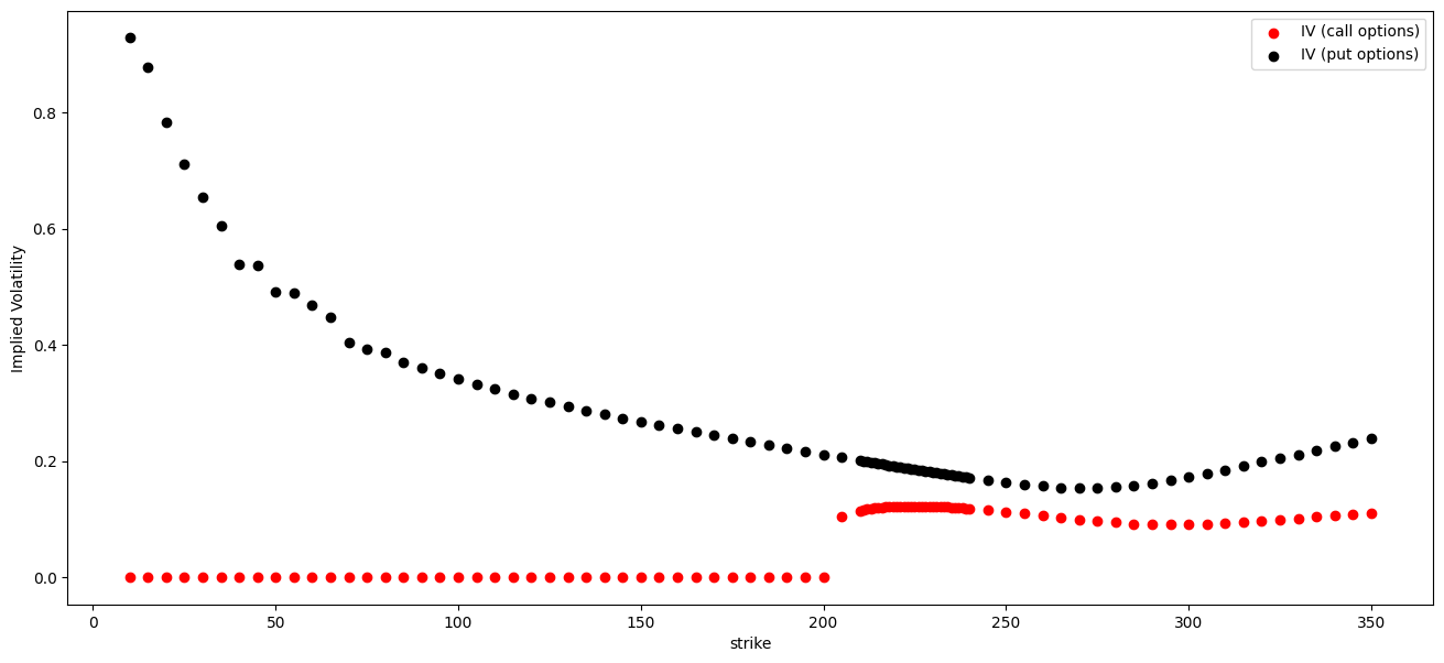
Plotting these implied volatilities across strikes gives us the implied volatility skew. For the shape of volatility smile, it should be a symmetry convex curve. But from the above chart, the implied volatility curve slopes downward to the right. This is referred to the skew, which means that options with low strikes have higher implied volatilities than those with higher strikes. The smile is not symmetry. The skew of a distribution is a measure of its asymmetry. Although the volatility skew is dynamic, in equity markets it is almost always a decreasing function of the strike. Other asset classes such as FX and commodities have differently shaped skews.
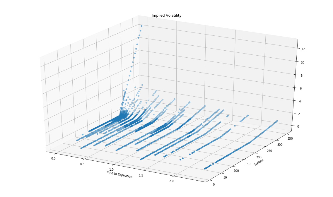
From the above chart, we can see the implied volatility for put options is higher than call options. Usually, put options trade for a higher price than call options, because traders place more risk in the short put positions, which raises the amount of reward they require to sell the position. Higher option prices signify an increase in risk and are represented by higher implied volatility levels derived from the option pricing model. Then we scattered all the implied volatilities of contracts across all the strikes.
# Get option contracts
start_date = datetime(2017, 8, 15)
spy = qb.AddEquity('SPY', resolution=Resolution.Daily)
spy.VolatilityModel = StandardDeviationOfReturnsVolatilityModel(2)
contract_symbols = qb.OptionChainProvider.GetOptionContractList(spy.Symbol, start_date)

# Subscribe to option contracts' data
symbols = []
for symbol in contract_symbols:
    contract = qb.AddOptionContract(symbol, resolution=Resolution.Daily, fillDataForward = False)
    contract.PriceModel = OptionPriceModels.BjerksundStensland()
    symbols.append(contract.Symbol)

# history request for IV
requests = []
for security in sorted(qb.Securities.Values, key=lambda x: x.Type):
    for subscription in security.Subscriptions:
        requests.append(HistoryRequest(subscription, security.Exchange.Hours, qb.StartDate-timedelta(1), qb.StartDate))
history = qb.History(requests)

df = pd.DataFrame()
done_symbol = []
for slice in history:
    underlying_price = None

    # Update the security with QuoteBars information
    for bar in slice.QuoteBars.Values:
        symbol = bar.Symbol
        if symbol in done_symbol:
            continue
        done_symbol.append(symbol)
        security = qb.Securities[symbol]
        security.SetMarketPrice(bar)

        if security.Type == SecurityType.Equity:
            underlying_price = security.Price
            continue

        # Create the Option contract
        contract = OptionContract.Create(symbol, symbol.Underlying, bar.EndTime, security, underlying_price)
        # Evaluate the price model to get the IV
        result = security.PriceModel.Evaluate(security, None, contract)
        # Append the data to the DataFrame
        data = {
            "IV" : result.ImpliedVolatility,
            "Strike" : contract.Strike,
            "Time till expiry (days)" : (contract.Expiry - bar.EndTime).days
        }
        index = [symbol.Value]
        df = pd.concat([df, pd.DataFrame(data, index=index)])

x = df["Time till expiry (days)"]
y = df.Strike
z = df.IV
fig = plt.figure(figsize=(20,11))
ax = fig.add_subplot(111, projection='3d')
ax.view_init(20,10)
ax.scatter(x,y,z)
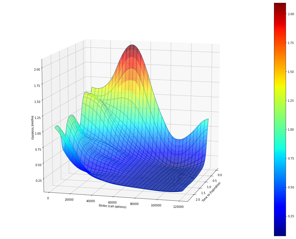
Volatility Surface
By fixing the maturity and looking at the implied volatilities of European options on the same underlying but different strikes, we obtain the implied volatility skew or smile. The volatility surface is the three-dimensional surface when we plots the market implied volatilities of European options with different strikes and different maturities.
Through the interpolation method, we can generate the implied volatility surface of SPY options for both put and call options as follows:
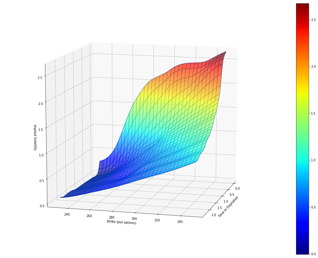
The Reason for Volatility Skew
The volatility skew reveals that for put options, implied volatility is higher for deep OTM options and is decreasing as it moves toward ITM options. For call options, the implied volatility is higher for deep ITM options and is decreasing as it moves toward OTM options. From the demand and supply degree, the skew reflects that investors are more willing to buy deep OTM puts and ITM calls. Why there is volatility skew in the market?
First, the majority of the equity positions are long. Investors usually have two ways to hedge those long positions risks: Buying downside puts or selling upside calls. The increase in demand create increases in the price of downside puts and decreases in the price of upside calls. The volatility is a reflection of options price. Therefore the volatility of in-the-money put is higher and the volatility of in-the-money call is lower.
The second reason for volatility skew is that the market moves down faster than it moves up. The downside market move is riskier than the upside move. Thus the price of OTM puts is higher than OTM calls.
Summary
In this chapter, we discussed the historical volatility and the implied volatility. The historical volatility of an asset is the statistical measure we know as the standard deviation of the stock return series. The implied volatility of the same asset, on the other hand, is the volatility parameter that we can infer from the prices of traded options written on this asset. In contrast to historical volatility, which looks at fluctuations of asset prices in the past, implied volatility looks ahead. The two volatilities do not necessarily coincide, and although they may be close, they are typically not equal.
Now we know the constant volatility assumption in Black-Sholes-Merton model is not applicable in the real market because there is volatility skew for most options. In next chapter, we will introduce some volatility models to capture the volatility skew in options pricing.
Reference
- Options Pricing: Intrinsic Value And Time Value, Jean Folger, Online Copy
ON THIS PAGE
Share


QuantConnect™ 2022. All Rights Reserved