Introduction
In the last chapter, we modeled the stock price with the Geometric Brownian motion. The logarithm of return follows the normal distribution . It means the logarithm of stock price follows the normal distribution . Based on this basic assumption, in this chapter, we will talk about a famous option pricing model: Black Scholes Merton Model.
Determinants of Option Price
In different kinds of asset pricing model like bond pricing, enterprise valuation, the most commonly used valuation method is to calculate the present value of the expected cash flows of that asset. But options have some characteristics that are different from the common asset. For example, the options value depends on its underlying asset. In addition, the cash flow on options are not constant over periods but depends on the occurrence of specific events which are not predictable. In fact, the value of the option is determined by lots of variables.
- The underlying price: Change in the value of the underlying asset is the most important factor which affects the options price. For the call option, holders can earn profit from the price rising and put option holders earn profits from the price decline. Therefore, call options become more valuable as the underlying prices increase while the put options will become less valuable.
- The volatility of the underlying asset: Volatility is a measure of the degree of fluctuation of the underlying stock price. It is a forward volatility, which means it is a prediction of how much the stock price of the underlying will move in the future over a certain period of time. The higher the predicted volatility is, the higher the probability that the underlying price will move a lot. Thus the greater will the value of the option is both for calls and puts. We will further discuss different types of volatilities in the subsequent tutorials.
- The strike price of the option: Call options gain profit when stock prices greater than the strike, it is easy to understand that the higher the strike price is for the call option, the fewer profits the holder can get, the less valuable of the call option. Thus for the put options, options with higher strike price are more valuable.
- Time to expiration: If the current date is t, the expiration date of the option contract is T. Then the time to expiration is T-t. For v=both call and put options, the longer time to expiration means there are more changes for the function of stocks prices, and higher probability for the option holders to gain profits from price movement.
- The risk-free interest rate: As interest rates increase, the expected return required by investors from the stock tends to increase. On the other hand, the present value of discounted cash flow will decrease. Thus the increase in interest rate will increase the call option price and will decrease the put option price.
- The dividend yield: After the dividends paid, the share price of the stock will decrease. During the options holding period, the decline in underlying price is unfavorable for call options holder. Therefore, the increase in dividend yield will decrease the price of call options and increase the price of put options.
Factors in BSM model
After we get an intuition about affecting factors of the options price, we will introduce the BSM option pricing model. The Black-Scholes model for pricing stock options was developed by Fischer Black, Myron Scholes and Robert Merton in the early 1970’s.
First, we introduce the factors in the model. For all the factors listed below, only volatility is not known. There are many types of volatilities. Then which volatility should be used is a critical question in option pricing model. We will further discuss this part in the next few chapters.
| Factors in the model | Symbol |
|---|---|
| Stock Price | S |
| Strike Price | K |
| Time to Expiration | T-t |
| Interest Rates | r |
| Future Volatility of the underlying Stock | σ |
class BsmModel:
    def __init__(self, option_type, price, strike, interest_rate, expiry, volatility, dividend_yield=0):
        self.s = price            # Underlying asset price
        self.k = strike           # Option strike K
        self.r = interest_rate    # Continuous risk fee rate
        self.q = dividend_yield   # Dividend continuous rate
        self.T = expiry           # time to expiry (year)
        self.sigma = volatility   # Underlying volatility
        self.type = option_type   # option type "p" put option "c" call option
There are some details we need to pay attention to about the input of BSM model. Firstly, the model works in continuous time, rather than discrete time. Therefore the risk-free rate r has to be modified to the continuous form. Secondly, the time to expiration should be converted to year. The volatility is the annual volatlity.
Model Assumptions
The market assumptions behind the Black–Scholes formula for pricing European options are as follows:
- The volatility of the underlying assets is constant over time
- The underlying asset price follows the lognormal distribution, this means that the log-returns of stock prices are normally distributed
- The underlying asset can be traded continuously
- The underlying stock does not pay dividends during the option's life. But the basic Black-Scholes model was later adjusted for dividends, here we demonstrate the later version with dividend yields.
- There are no transaction costs or taxes
- All securities are perfectly divisible, meaning that it is possible to buy any fraction of a share
- The risk-free rate of interest, r, is constant and the same for all maturities
Model Equations
The derivation of the Black-Scholes model is beyond the scope of this research, we only show the formula here. The basic principle is based on the idea of creating a portfolio of the underlying asset and the riskless asset with the same cash flows and hence the same cost as the option being valued. Then we get the Black–Scholes–Merton differential equation. The solutions to the differential equation are the Black-Scholes-Merton formulas for the price of European call and put options
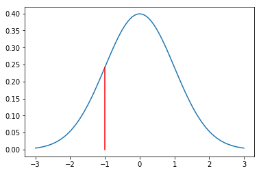
N(x) is the cumulative probability distribution function for a variable with a standard normal distribution. It can be calculated by the integral of the probability density function of standard normal distribution from 0 to x. In Python, you can use the norm.pdf(x) in spicy.stats library. For the following chart, we plot the probability density curve of the standard normal distribution. For example, N(-1) is the area of the left hand of the red line under the curve.
import scipy.stats as sp
mu = 0
variance = 1
x = np.linspace(mu-3*variance,mu+3*variance, 100)
y = [sp.norm.pdf(i) for i in x]
plt.plot(x,y)
d = [-1]
plt.plot(d*100,np.linspace(0,sp.norm.pdf(d), 100))
Then in our BSM model class, we will calculate the European call and put option prices by using BSM formula.
import scipy.stats as sp

class BsmModel:
    def __init__(self, option_type, price, strike, interest_rate, expiry, volatility, dividend_yield=0):
        self.s = price            # Underlying asset price
        self.k = strike           # Option strike K
        self.r = interest_rate    # Continuous risk fee rate
        self.q = dividend_yield   # Dividend continuous rate
        self.T = expiry           # time to expiry (year)
        self.sigma = volatility   # Underlying volatility
        self.type = option_type   # option type "p" put option "c" call option

    def n(self, d):
        # cumulative probability distribution function of standard normal distribution
        return sp.norm.cdf(d)

    def dn(self, d):
        # the first order derivative of n(d)
        return sp.norm.pdf(d)

    def d1(self):
        return (log(self.s / self.k) + (self.r - self.q + self.sigma ** 2 * 0.5) * self.T) / (self.sigma * sqrt(self.T))

    def d2(self):
        return (log(self.s / self.k) + (self.r - self.q - self.sigma ** 2 * 0.5) * self.T) / (self.sigma * sqrt(self.T))

    def bsm_price(self):
        d1 = self.d1()
        d2 = d1 - self.sigma * sqrt(self.T)
        if self.type == 'c':
            return exp(-self.r*self.T) * (self.s * exp((self.r - self.q)*self.T) * self.n(d1) - self.k * self.n(d2))
        if self.type == 'p':
            return exp(-self.r*self.T) * (self.k * self.n(-d2) - (self.s * exp((self.r - self.q)*self.T) * self.n(-d1)))
        print ("option type can only be c or p")

a = BsmModel('c', 42, 35, 0.1, 90.0/365, 0.2)
a.bsm_price()
For a call option which expires in 90 days and no dividends paid, the underlying price is $42, the strike is $35, the risk-free rate is 0.1, the volatility is 0.2. The price of this option is $7.88.
Summary
This tutorial discussed factors affecting the options price and introduced a famous option pricing model including input parameters, assumptions and the formula.
ON THIS PAGE
Share


QuantConnect™ 2022. All Rights Reserved