


 Share New Research


Introduction
Aggregate sales growth (ASG) measures how fast revenue is expanding across the average US public company, weighted by size. Garfinkel, Hribar, and Hsiao (2025) document a negative relationship between this aggregate and future market excess returns, which they trace to intensified market competition that squeezes future earnings and to investors over-extrapolating the growth. This strategy turns that finding into a monthly market-timing rule that rotates between the SPY and the BIL, sizing the Equity leg by mean-variance optimization. The signal itself is rebuilt each month from the cross-section of US non-financial common stocks using Morningstar fundamentals. Over July 2021 to July 2026, the strategy earned a 0.753 Sharpe ratio, outperforming a buy-and-hold position in the SPY.
Background
Sales are the least discretionary line in an income statement, so their growth carries information about future earnings. Garfinkel et al. (2025) attribute the negative relationship to two channels. The competition channel holds that high aggregate sales growth reflects intensified market competition rather than stronger fundamentals, and that competition compresses future profit margins, so aggregate earnings weaken and the market's subsequent excess return is lower. The mispricing channel holds that investors read the fast growth as a sign of strong future profitability and over-extrapolate it, lifting prices that later correct when earnings disappoint. Because the effect lives in the aggregate rather than in the cross-section, it times the market as a whole instead of ranking individual stocks, which makes a rotation between a risky and a risk-free asset the natural way to trade it.
Aggregate Sales Growth
The signal is built one firm at a time from each firm's one-year sales growth. Aggregating those firm-level readings by size gives the month's signal,
\[ \text{ASG}_t = \frac{\sum_i g_{i,t} \, M_{i,t}}{\sum_i M_{i,t}}, \]
where \( g_{i,t} \) is firm \( i \)'s one-year sales growth and \( M_{i,t} \) is its market capitalization in month \( t \), and the sums run over the eligible cross-section. That cross-section is the current month's US common stocks outside the financial and real estate sectors, which are excluded because sales are not a meaningful operating quantity for them. Firm-level growth is winsorized at the 1st and 99th percentiles of that month's cross-section before aggregating, so a single extreme growth reading cannot swing the aggregate.
Return Forecast
The aggregate becomes a forecast through an ordinary least squares regression that predicts the market's next-month excess return from the current aggregate, refit each month on an expanding window of all months through \( t \),
\[ \hat{R}_{t+1} = \hat{\alpha}_t + \hat{\beta}_t \, \text{ASG}_t, \]
where \( \hat{R}_{t+1} \) is the predicted excess return for the coming month, \( \hat{\alpha}_t \) is the fitted intercept, and \( \hat{\beta}_t \) is the fitted slope on the aggregate. The regression pairs each month's aggregate with the following month's realized excess return, so the negative relationship shows up as a negative \( \hat{\beta}_t \).
Position Sizing
A mean-variance investor judges a portfolio by trading off expected return against risk, valuing next month's portfolio by its expected return minus a penalty proportional to its variance. How heavily that variance counts is set by the investor's risk aversion. Maximizing this objective over the split between the market and the risk-free asset gives a closed-form Equity weight,
\[ w_t = \frac{\hat{R}_{t+1}}{\gamma \, \hat{\sigma}^2_{t+1}}, \]
where \( \gamma \) is the coefficient of relative risk aversion and \( \hat{\sigma}^2_{t+1} \) is the variance of monthly market excess returns over the trailing 10 years. The weight rises with the forecast excess return and falls with both the market's variance and the investor's risk aversion. The strategy sets \( \gamma = 3 \), one of the two risk-aversion coefficients Garfinkel et al. (2025) evaluate, and adopts their restriction that the weight stay positive and not exceed 150%, so \( w_t \) is confined to the interval \( [0, 1.5] \). It therefore never shorts the market and never levers beyond 150%. The remaining \( 1 - w_t \) goes to the T-bill leg, which turns negative when the forecast justifies leverage and then represents the financing cost of the levered position.
Implementation
To implement this strategy, we start by adding the risky and risk-free assets in the initialize. SPY represents the risky leg and the BIL represents the risk-free leg.
self._spy = self.add_equity("SPY", Resolution.DAILY, leverage=3)
self._bil = self.add_equity("BIL", Resolution.DAILY, leverage=3)
We then add some members we'll need to make trading decisions. The algorithm keeps the running aggregate sales growth series, the realized excess-return series that the regression fits against, and a 120-month variance of those excess returns.
self._firm_data = {}
self._asg = pd.Series()
self._market_return = RateOfChange(1)
self._excess_returns = pd.Series()
self._gamma = 3
lookback_years = 10
self._var = Variance(lookback_years * 12)
To get the fundamental data we need, we add a fundamental universe. The portfolio rebalances monthly, so we also add a Scheduled Event and configure both the universe selection and rebalance logic to run at the start of each month.
# Add a universe that runs selection at the start of each month.
date_rule = self.date_rules.month_start("SPY")
self.universe_settings.schedule.on(date_rule)
self._universe = self.add_universe(self._select_assets)
# Add a Scheduled Event to rebalance the portfolio each month.
self.schedule.on(date_rule, self.time_rules.at(8, 0), self._rebalance)
We need to warm up the variance indicator and gather samples to fit the regression model, so we add a warm-up period.
self.set_warm_up(timedelta((lookback_years+1)*365))Each month, the _select_assets method first selects the eligible cross-section. It keeps US primary-share common stocks outside the Financial Services and Real Estate sectors, and stores each firm's one-year revenue growth and market capitalization. The method then returns an empty list because the algorithm never trades these stocks. The universe selection function only exists to gather the data needed to calculate ASG.
def _select_assets(self, fundamentals: List[Fundamental]) -> List[Symbol]:
    self._firm_data = {
        f.symbol: (f.operation_ratios.revenue_growth.one_year, f.market_cap)
        for f in fundamentals
        if (f.company_reference.country_id == "USA" and
            f.security_reference.is_primary_share and
            f.security_reference.security_type == "ST00000001" and
            f.asset_classification.morningstar_sector_code not in (MorningstarSectorCode.FINANCIAL_SERVICES, MorningstarSectorCode.REAL_ESTATE))
    }
    return []
The _rebalance method starts by recording the month that just closed. It then calculates the SPY's excess monthly return using the risk-free rate. It records the excess return and also pushes it through the variance indicator.
# Get the month that just ended.
month = pd.Period(self.time, freq="M") - 1
# Update the excess return history.
if self._market_return.update(self.time, self._spy.price):
    excess_return = self._market_return.current.value - self.risk_free_interest_rate_model.get_interest_rate(self.time) / 12
    self._excess_returns[month] = excess_return
    self._var.update(self.time, excess_return)
The _rebalance method then goes on to calculate ASG, which is the market-cap-weighted average of the winsorized firm-level growth rates.
firms = pd.DataFrame.from_dict(self._firm_data, orient="index", columns=["growth", "market_cap"]).dropna(subset=["growth"])
growth = firms["growth"].clip(*firms["growth"].quantile([0.01, 0.99]))
caps = firms["market_cap"]
usable = caps.notna() & (caps > 0)
if usable.any():
    self._asg[month] = np.average(growth[usable], weights=caps[usable])
Shifting the aggregate forward one month and aligning it against the realized excess returns pairs each month's ASG with the excess return it is meant to predict. Fitting a first-degree polynomial to those pairs gives the intercept and slope, which turn the current month's ASG into next month's forecast of excess returns.
# Regress this month's excess return on last month's ASG.
X, y = self._asg.shift(1, freq="M").align(self._excess_returns, join="inner")
alpha, beta = np.polynomial.polynomial.polyfit(X, y, 1)
# Forecast this month's excess return.
forecast_r = alpha + beta * self._asg.get(month)
The forecast and the trailing variance then produce the Equity weight, which we clip to the \( [0, 1.5] \) interval before rebalancing both positions to their target weights.
w_star = np.clip(forecast_r / (self._gamma * self._var.current.value), 0, 1.5)
self.set_holdings([PortfolioTarget(self._spy, w_star), PortfolioTarget(self._bil, 1 - w_star)])
Results
We backtested the strategy over July 2021 to July 2026, and it earned a 0.753 Sharpe ratio. In contrast, a buy-and-hold position in the SPY over the same time period achieved a 0.412 Sharpe ratio. Therefore, the strategy outperformed the benchmark. However, much of the gain over the S&P 500 comes from the algorithm reducing its exposure to Equities during the 2022 selloff of the Ukraine war. The stimulus-driven sales surge of 2021 signaled low expected returns for 2022, yet the edge is hard to separate from fortunate timing.
We ran a parameter optimization job to test the sensitivity of the chosen parameters. We varied the risk-aversion coefficient from 1 to 5 in steps of 1, and we varied the length of the variance-estimation window from 8 to 12 years in steps of 1 year. Of the 25 parameter combinations, all 25 (100%) produced a greater Sharpe ratio than the benchmark. The following image shows the heatmap of Sharpe ratios for the parameter combinations:
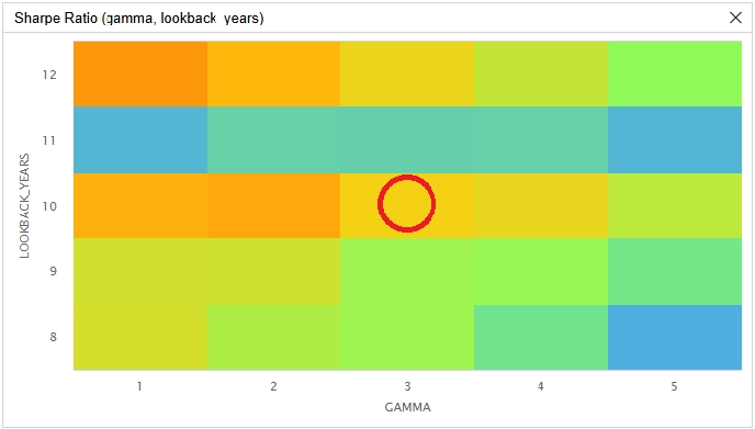
The red circle in the preceding image identifies the parameters we chose as the strategy's default. We chose a risk-aversion coefficient of 3 and a 10-year variance window because both are settings from Garfinkel et al. (2025). That combination produced a 0.753 Sharpe ratio, above the grid's 0.670 mean but below its 0.807 maximum. The maximum sits at the corner of the searched range, at a coefficient of 1 and a 12-year window, so we kept the paper's interior values rather than the Sharpe-maximizing cell.
The risk-aversion coefficient shows a mild tilt, with the Sharpe ratio tending to fall as the coefficient rises, by roughly 0.1 to 0.2 across most rows. That direction follows from the weight formula, since a lower coefficient scales every target weight up and holds the risk exposure at or near its 150% cap more often. Because a levered position and its unlevered counterpart share almost the same Sharpe ratio, and the spread is small and in-sample, we read this as a sample-specific tilt rather than a robust preference for lower risk aversion.
The variance window behaves very differently, swinging erratically rather than trending. The 11-year window sits near 0.55 at every coefficient, far below its 10-year and 12-year neighbors, which range from roughly 0.65 to 0.81. A one-year change in a decade-long window cannot plausibly move the Sharpe ratio that far, because those rolling variances are highly correlated and slow-moving, so we attribute the swing to sampling noise. With the grid maximum also sitting at the corner of the searched range, we do not attach an economic story to the peak or treat the surface's gradient as an established effect.
Across the grid, every combination beat the benchmark, so the strategy's edge over holding the SPY does not depend on the exact risk aversion or variance window. Beyond that robustness, the surface reads more as a caution than a confirmation, because its best cells sit at the boundary of the searched range and one window setting swings the Sharpe ratio erratically. Both point to performance that is unstable in these parameters over a five-year sample.
Future research could sharpen the forecast by combining ASG with aggregate earnings growth and standard macroeconomic return predictors. The sizing could also react faster to risk, since replacing the slow decade-long variance with a more responsive volatility model would shrink the position when markets turn. The signal itself could also extend beyond the SPY to international Equity markets that show the same predictability.
References
- Garfinkel, J. A., Hribar, P., & Hsiao, L. (2025). Aggregate Sales Growth and Stock Market Returns (Working paper). SSRN. https://papers.ssrn.com/sol3/papers.cfm?abstract_id=5066654


Dhennis
Very nice
Derek Melchin
The material on this website is provided for informational purposes only and does not constitute an offer to sell, a solicitation to buy, or a recommendation or endorsement for any security or strategy, nor does it constitute an offer to provide investment advisory services by QuantConnect. In addition, the material offers no opinion with respect to the suitability of any security or specific investment. QuantConnect makes no guarantees as to the accuracy or completeness of the views expressed in the website. The views are subject to change, and may have become unreliable for various reasons, including changes in market conditions or economic circumstances. All investments involve risk, including loss of principal. You should consult with an investment professional before making any investment decisions.
To unlock posting to the community forums please complete at least 30% of Boot Camp.
You can continue your Boot Camp training progress from the terminal. We hope to see you in the community soon!