


 Share New Research


Introduction
Pairs trading buys one stock and shorts a similar one when the gap between their prices widens, betting that the gap will close. Yang, Tsai, Shyu and Chang (2016) time these trades with a model in which the gap reverts toward a mean that switches between two regimes. Among S&P 500 stocks, their regime-switching rule earned higher returns than the classic distance rule. The strategy in this research post trades their model on the five most closely matched pairs of S&P 500 stocks each month, using the US ETF Constituents and US Fundamental datasets. From November 2021 to November 2026, it earned a 5.56% compounding annual return with a beta of 0.01.
Background
Pairs trading rests on the idea that companies with similar businesses respond to the same economic news, so their stock prices tend to move together. When the gap between two such prices widens without a lasting change in either business, the gap tends to close again. A position that buys the stock that fell and shorts the one that rose profits when the gap closes, regardless of what the overall market does.
Pair Formation
Following Gatev et al. (2006), the strategy measures how closely two stocks move together with the sum of squared differences (SSD) between their normalized prices over the past year,
\[ SSD_{A,B} = \sum_{t=1}^{252} \left( \tilde{P}^A_t - \tilde{P}^B_t \right)^2 \quad \text{with} \quad \tilde{P}^i_t = \prod_{\tau=1}^{t} \left( 1 + r^i_\tau \right), \]
where \( \tilde{P}^i_t \) is the price of stock \( i \) rebased to start at 1 and \( r^i_\tau \) is its return on day \( \tau \). At the start of each month, the strategy computes the SSD of every pair of S&P 500 stocks and selects the five pairs with the smallest SSD as the pairs that can open positions that month. Some companies have two share classes in the index, such as Alphabet's GOOG and GOOGL. Their prices move almost identically, so the strategy keeps only the share class with larger weight in the S&P 500.
Regime Switching
A regime-switching model lets a time series switch between a few distinct states, called regimes, that can't be observed directly. Each regime has its own parameters, and the model infers the probability of each regime from the data. The time series in this strategy is each pair’s spread, which is the difference between the log prices of its two stocks,
\[ s_t = \ln P^A_t - \ln P^B_t, \]
where \( P^A_t \) and \( P^B_t \) are the closing prices of stocks A and B on day \( t \).
The Vasicek (1977) model describes a spread that reverts toward a long-run mean at a constant speed. Yang et al. (2016) let its parameters switch between two regimes that follow a Markov chain, as in Hamilton (1989), because spreads can alternate between calm and turbulent periods. Each day's change in the spread follows
\[ \Delta s_t = \kappa_{S_t} \left( \theta_{S_t} - s_{t-1} \right) + \varepsilon_t \quad \text{with} \quad \varepsilon_t \sim N\left( 0, \sigma^2_{S_t} \right), \]
where \( S_t \) is the regime on day \( t \) and \( \varepsilon_t \) is the day's shock. In each regime, \( \kappa \) is the speed of mean reversion, \( \theta \) is the long-run mean and \( \sigma \) is the volatility of the shocks. The regime moves from \( j \) to \( i \) with probability \( p_{ij} \), and the strategy estimates all eight parameters each day by maximum likelihood over the past year of the spread.
Trading Rule
Each day, the strategy predicts the regime from the transition probabilities and the regime probabilities at the previous close,
\[ P\left( S_t = i \mid \mathcal{F}_{t-1} \right) = \sum_{j=1}^{2} p_{ij} \, P\left( S_{t-1} = j \mid \mathcal{F}_{t-1} \right), \]
where \( \mathcal{F}_{t-1} \) is the information available through day \( t-1 \). With the parameters of the more likely regime, it forecasts the spread as
\[ F_t = s_{t-1} + \kappa \left( \theta - s_{t-1} \right) \]
and opens a position when the spread closes far from that forecast. If \( s_t - F_t \ge 2 \sigma \), stock A has become expensive relative to stock B, so the strategy shorts A and buys B. If \( s_t - F_t \le -2 \sigma \), stock A has become cheap relative to stock B, so the strategy buys A and shorts B. Yang et al. (2016) set this critical value at 1.96, the two-sided 5% critical value of the normal distribution. To avoid overfitting, we round it up to 2 standard deviations, which corresponds to a probability of about 95%. Because the signal uses closing prices, the strategy trades at the next day's open.
The half-life of a regime is the number of days it takes to close half of the gap between the spread and its mean. A position closes when the spread returns to the forecast it overshot or after one half-life of the predicted regime,
\[ h = \frac{\ln 0.5}{\ln \left| 1 - \kappa \right|}, \]
where \( h \) is the half-life in days. When \( \left| 1 - \kappa \right| \ge 1 \), the regime doesn't revert, so the strategy ignores the signal.
Position Sizing
The portfolio can hold up to five pairs at a time. When fewer than five pairs are open, the strategy puts the unused cash in BIL, an ETF of 1- to 3-month Treasury bills that serves as the risk-free asset.
Implementation
To implement this strategy, we start by adding BIL and the universe in the initialize method. The universe is a chained universe that passes SPY's holdings from an ETF constituents universe to a fundamental universe selection function. The schedule universe setting runs that selection on the first trading day of each month. We also add a Scheduled Event that rebalances the portfolio at 8 AM Eastern Time (ET) each trading day.
# Add a risk-free asset to consume unused cash.
self._bil = self.add_equity('BIL', Resolution.DAILY)
# Add a universe of US Equities that selects pairs from SPY constituents at the start of each month.
self._weight_by_symbol = {}  # The weight of each stock in the ETF.
self.universe_settings.resolution = Resolution.DAILY
self.universe_settings.schedule.on(self.date_rules.month_start('SPY'))
self._universe = self.add_universe(self.universe.etf('SPY', universe_filter_func=self._select_holdings), self._form_pairs)
# Add a Scheduled Event to rebalance the portfolio.
self.schedule.on(self.date_rules.every_day('SPY'), self.time_rules.at(8, 0), self._rebalance)
The constants at the top of the file set the one-year window, the standard deviations threshold, and the position sizes.
SESSIONS_PER_YEAR = 252
STD_DEVIATIONS = 2
MAX_PAIRS = 5
LEG_WEIGHT = 0.75 / MAX_PAIRS
The _select_holdings universe selection function saves the weight of each stock in SPY and passes every holding to the _form_pairs method. The _form_pairs method then groups the stocks by their company identifier and keeps the share class with the larger weight in SPY.
def _form_pairs(self, fundamentals: List[Fundamental]) -> List[Symbol]:
    # Some stocks in the ETF represent the same company. For each case, only use the stock with the largest weight in the ETF.
    company_by_symbol = {f.symbol: f.company_reference.company_id for f in fundamentals}
    symbols_by_company = {}
    for symbol in self._weight_by_symbol:
        symbols_by_company.setdefault(company_by_symbol.get(symbol, str(symbol.id)), []).append(symbol)
    symbols = [
        min(group, key=lambda s: (-self._weight_by_symbol[s], s.value))
        for group in symbols_by_company.values()
    ]
Next, the method gets the trailing year of daily returns. It rebases each stock's prices to start at 1 and computes the SSD of every pair at once with matrix algebra.
# The smallest sums of squared differences of the normalized prices (paper Eq. 15).
#  - Get the historical closing prices for each stock.
closes = self.history(symbols, SESSIONS_PER_YEAR + 1, Resolution.DAILY, fill_forward=False).close.unstack(0).dropna(axis=1)
normalized = (closes.pct_change().iloc[1:] + 1).cumprod().values.T
squared_norms = (normalized ** 2).sum(axis=1)
#  - Compute the sum of squared differences for every pair at once (SSD between stocks i and j).
ssd = squared_norms[:, None] + squared_norms[None, :] - 2 * normalized @ normalized.T
ssd[np.tril_indices(len(ssd))] = np.inf
It then saves the five pairs with the smallest SSD and returns their stocks as the universe, along with the stocks of the pairs that the portfolio still holds.
#  - Pick the pairs whose normalized price paths over the past 252 days have the smallest SSD.
closest = (divmod(int(k), len(ssd)) for k in np.argsort(ssd, axis=None)[:MAX_PAIRS])
self._formed_pairs = [(closes.columns[i], closes.columns[j]) for i, j in closest if np.isfinite(ssd[i, j])]
# Set the universe to the stocks in the new pairs and the pairs we're already holding.
return list({s for pair in self._formed_pairs for s in pair} | {s for pair in self._position_by_pair for s in pair})
On the first trading day of each month, the _rebalance method makes the month's new pairs the ones that can open. Each day, it then computes the log spread of every eligible or open pair over the past year.
def _rebalance(self) -> None:
    # On each new month, the month's closest pairs become the pairs that may open.
    if self.time.month != self._month:
        self._month = self.time.month
        self._eligible_pairs, self._formed_pairs = self._formed_pairs, []
    # Get the spread of each pair.
    pairs = list(dict.fromkeys(list(self._position_by_pair) + self._eligible_pairs))
    symbols = list({s for pair in pairs for s in pair})
    closes = self.history(symbols, SESSIONS_PER_YEAR + 2, Resolution.DAILY, fill_forward=False).close.unstack(0)
    spread_by_pair = {(a, b): np.log(closes[a]) - np.log(closes[b]) for a, b in pairs}
The method first closes any pair that contains a delisted stock, a spread that is back at the forecast it overshot, or has been held for a period of one half-life.
# Scan for exits.
for pair, position in list(self._position_by_pair.items()):
    position.sessions_held += 1
    if (any(self.securities[s].is_delisted for s in pair) or
        position.has_reverted(spread_by_pair[pair].iloc[-1]) or
        position.sessions_held >= position.half_life):
        del self._position_by_pair[pair]
It then scans the month's pairs for entries until five pairs are open. A pair opens when the _signal method finds a shock beyond the band and the predicted regime is mean-reverting.
# Scan for entries.
for pair in self._eligible_pairs:
    if len(self._position_by_pair) >= MAX_PAIRS:
        break
    if pair in self._position_by_pair or any(self.securities[s].is_delisted for s in pair):
        continue
    direction, forecast, half_life = self._signal(spread_by_pair[pair])
    if not direction or math.isinf(half_life):
        continue
    self._position_by_pair[pair] = PairPosition(direction, forecast, half_life)
After the scans, the _rebalance method gives each open pair one-fifth of the portfolio and puts the unused cash in BIL.
# Calculate portfolio weights of each stock in each pair.
weight_by_symbol = defaultdict(float)
for (a, b), position in self._position_by_pair.items():
    weight_by_symbol[a] += position.direction * LEG_WEIGHT
    weight_by_symbol[b] -= position.direction * LEG_WEIGHT
# If there is unused cash, put it in the risk-free asset.
weight_by_symbol[self._bil] = (MAX_PAIRS - len(self._position_by_pair)) / MAX_PAIRS
It then rebalances only the securities whose target weights changed, so the legs of an open pair keep their positions until the pair closes. The orders are placed before the open, so they fill at the opening price as market on open orders.
# Place trades to rebalance the portfolio.
targets = [
    PortfolioTarget(s, weight_by_symbol.get(s, 0)) for s in set(weight_by_symbol) | set(self._target_by_symbol)
    if weight_by_symbol.get(s, 0) != self._target_by_symbol.get(s, 0)
]
if targets:
    self.set_holdings(targets)
# Save the target weights, so we know if we need to place orders next time.
self._target_by_symbol = {s: w for s, w in weight_by_symbol.items() if w}
The _signal helper method, which the entry scan calls for each pair, fits the two-regime model to the daily changes in the spread over the trailing year before the latest close. A regression of each day's change on the previous day's spread is the discrete form of the Vasicek model, with an intercept of \( \kappa \theta \) and a slope of \( -\kappa \). To fit it, the method searches for the parameters that maximize the model's likelihood with the BFGS method of SciPy's minimize function.
def _signal(self, spread: pd.Series) -> tuple:
    """Signal Z, one-day forecast F and half-life of the latest session (paper Eqs. 16-17); Z is 0 when
    there is none."""
    # Fit the two-regime model to the spreads before the latest session (paper Eqs. 2-8).
    #  - Regress each day's change in the spread on the previous day's spread. The intercept, slope and noise level switch between two regimes.
    window = spread.values[:-1]
    lagged, changes = window[:-1], np.diff(window)
    #  - Find the parameters that maximize the likelihood with a BFGS search, starting from an OLS fit on each half of the window.
    estimate = minimize(lambda x: -hamilton_filter(x, lagged, changes)[0], starting_values(window), method="BFGS").x
It then runs the filter with the estimated parameters to get the regime probabilities of the last day in the window. If the search fails to reach a finite estimate, the method skips the pair.
#  - Run the filter with the estimate to get its log-likelihood and the regime probabilities of the last day in the window.
log_likelihood, f1, f2 = hamilton_filter(estimate, lagged, changes)
# Skip pairs where the search fails to reach a finite estimate.
if not (math.isfinite(log_likelihood) and np.all(np.isfinite(estimate))):
    return 0, math.nan, math.nan
The method predicts the regime of the latest close by multiplying the transition probabilities by the regime probabilities of the previous day. It then reads the intercept, slope and volatility of the more likely regime.
# Predict the regime of the latest session (paper Eq. 7).
#  - Convert the estimates into the probability of staying in state 1 and the probability of leaving state 2.
p11, leave2 = 1 / (1 + np.exp(-estimate[6])), 1 / (1 + np.exp(estimate[7]))
#  - Weight the chances of reaching state 1 from each state by the regime probabilities of the last day in the window.
q1 = p11 * f1 + leave2 * f2  # prediction probability of state 1 for the latest session (Eq. 7)
#  - Get the intercept, slope and log noise level of the more likely regime.
a, b, log_sigma = estimate[:3] if q1 >= 1 - q1 else estimate[3:6]
With those parameters, it compares the latest spread with the regime's forecast and sets the band at 2 standard deviations of the regime's shocks.
# Compare the latest spread to the regime's forecast (paper Eqs. 16-17).
#  - Forecast the latest spread from the previous day's spread.
forecast = window[-1] + a + b * window[-1]
#  - Measure how far the latest spread is from the forecast.
shock = spread.values[-1] - forecast
#  - Set the band at the chosen number of standard deviations of the regime's noise.
band = STD_DEVIATIONS * np.exp(log_sigma)
The half-life comes from the slope, since \( 1 + b = 1 - \kappa \) is the share of a gap that remains after one day. The method returns the direction of the trade along with the forecast and the half-life.
# Calculate how many sessions the predicted regime takes to close half of a gap (infinite if it doesn't revert).
persistence = abs(1 + b)  # share of a gap left after one session in the predicted regime
half_life = math.log(0.5) / math.log(persistence) if 0 < persistence < 1 else math.inf
# Short the spread (-1) if the shock is above the band, or buy it (+1) if the shock is below the band.
return (-1 if shock >= band else (1 if shock <= -band else 0)), forecast, half_life
The likelihood comes from the hamilton_filter function in the regime_switching.py file of the project, which runs the filter that Hamilton (1989) introduced.
Results
From November 2021 to November 2026, the strategy earned a 5.56% compounding annual return with a beta of 0.01. Therefore, it achieved a positive return with effectively no exposure to the overall market.
We ran a parameter optimization job to test the sensitivity of the chosen parameters. We tested standard deviations from 1.8 to 2.2 in steps of 0.2. We also tested lookback periods from 8 to 16 months in steps of 2 months, which set the length of both the formation window and the estimation window. To avoid trading errors in the optimization backtests, we removed the strategy's leverage, so their returns are slightly lower than the original backtest's. All 25 parameter combinations earned a positive return with betas of 0.01 or less. The following image shows the heatmap of compounding annual returns for the parameter combinations:
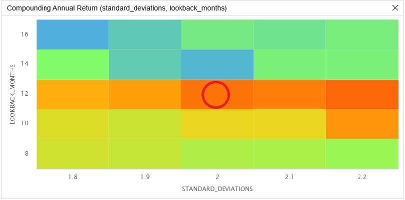
The red circle in the preceding image identifies the parameters we chose as the strategy's default. We chose a standard deviations threshold of 2 and a lookback period of 12 months because they're about the values that Yang et al. (2016) use.
The lookback period matters much more than the number of standard deviations. Averaged across band widths, the compounding annual return is 4.0% with a 12-month lookback and 3.1% with a 10-month lookback. It falls to 2.3% with an 8-month lookback and to 1.1% and 1.0% with lookbacks of 14 and 16 months. The effect of the band width depends on the lookback, since the return falls from 2.67% to 1.95% as the band widens with an 8-month lookback but peaks at the widest band with 10- and 12-month lookbacks.
The lookback sets the window that forms the pairs, so it decides which stocks pair up each month. The pairs are mostly utilities and apartment REITs, so a few lasting moves in single stocks can decide a run's result. From September 2024 to February 2025, four of the five 10-month runs lost money as Entergy rallied on power demand from data centers. Entergy shorts accounted for about half or more of each of those losses, while all five 12-month runs made money over the same months. Earlier in 2024, the 14-month runs lost money on CenterPoint as it fell after Hurricane Beryl. A plausible explanation for the sensitivity is that each lookback holds a different set of pairs, so its result depends on which stocks it happened to hold when moves like these came.
The strategy earned a positive return with almost no market exposure in every parameter combination we tested, and most of the backtest's return came from the pair trades rather than the Treasury bills that hold its idle capital. Its sensitivity to the lookback suggests that the result depends more on which stocks pair up than on the width of the band. Future research could pair stocks within each industry and hold pairs from several industries, as Yang et al. (2016) suggest, so that no single industry dominates the portfolio. It could also trade near the close with intraday data, so positions open on the day of the shock instead of at the next open. Finally, a cointegration test when the pairs form could screen out pairs whose spreads revert too slowly to trade, since the current check only requires some reversion in the predicted regime.
References
- Gatev, E., Goetzmann, W. N., & Rouwenhorst, K. G. (2006). Pairs trading: Performance of a relative-value arbitrage rule. The Review of Financial Studies, 19(3), 797-827. https://doi.org/10.1093/rfs/hhj020
- Hamilton, J. D. (1989). A new approach to the economic analysis of nonstationary time series and the business cycle. Econometrica, 57(2), 357-384. https://doi.org/10.2307/1912559
- Vasicek, O. (1977). An equilibrium characterization of the term structure. Journal of Financial Economics, 5(2), 177-188. https://doi.org/10.1016/0304-405X(77)90016-2
- Yang, J.-W., Tsai, S.-Y., Shyu, S.-D., & Chang, C.-C. (2016). Pairs trading: The performance of a stochastic spread model with regime switching-evidence from the S&P 500. International Review of Economics and Finance, 43, 139-150. https://doi.org/10.1016/j.iref.2015.10.036


Derek Melchin
The material on this website is provided for informational purposes only and does not constitute an offer to sell, a solicitation to buy, or a recommendation or endorsement for any security or strategy, nor does it constitute an offer to provide investment advisory services by QuantConnect. In addition, the material offers no opinion with respect to the suitability of any security or specific investment. QuantConnect makes no guarantees as to the accuracy or completeness of the views expressed in the website. The views are subject to change, and may have become unreliable for various reasons, including changes in market conditions or economic circumstances. All investments involve risk, including loss of principal. You should consult with an investment professional before making any investment decisions.
This discussion is closed