Dynamic Conversion Arbitrage on the Magnificent 7

Introduction

Conversion arbitrage is a classic Options trade that produces a fixed payoff by combining a long stock position with a long put and a short call at the same strike and expiry. This strategy hunts for conversions on the Magnificent 7 stocks whose annualized return exceeds a minimum threshold, opens the most attractive one, and dynamically swaps into a better conversion if one surfaces. It trades the Equities and their Options and parks idle capital in the SHV Treasury ETF. From January 2023 to June 2026 the strategy earned a 7.5% compounding annual return with a maximum drawdown of 1.1% and a portfolio beta of 0.017, a nearly market-neutral profile.

Background

Conversion arbitrage rests on put-call parity, the no-arbitrage relationship that ties together the prices of a stock, a call, and a put that share a strike and expiry.

Put-Call Parity and the Conversion

A conversion holds a long stock position, a long put, and a short call at the same strike and expiry. At expiry, the put and call together convert the stock into the strike regardless of where the stock trades, so the package pays a fixed amount and behaves like a bond. Put-call parity ties these prices together as

\[ S + P - C = K e^{-rT}, \]

where \( S \) is the stock price, \( C \) and \( P \) are the call and put prices, \( K \) is the strike, \( r \) is the risk-free rate, and \( T \) is the time to expiry. The left side is the cost of building the conversion and the right side is the strike, discounted to its present value. When the market prices the legs so that the conversion costs less than that present value, the trade captures a return above the risk-free rate. Because these Options expire within weeks, the present value of the strike is almost identical to the strike itself, so the strategy works with the strike directly.

The Annualized Return Surface

The strategy calculates each conversion's annualized return from executable prices, selling the call at its bid, buying the put at its ask, and buying the stock at its ask. That return is

\[ \text{AR} = \frac{(C - P) + (K - S)}{S \, t} \times 100, \]

where \( C \) is the call bid, \( P \) the put ask, \( S \) the stock ask, \( K \) the strike, and \( t \) the time to expiry in years. The numerator is the profit per share the conversion captures, namely the Option net credit \( C - P \) plus the gap between the strike and the stock price. Plotting this annualized return across every strike and expiry traces a surface whose peaks mark the conversion(s) with the greatest return.

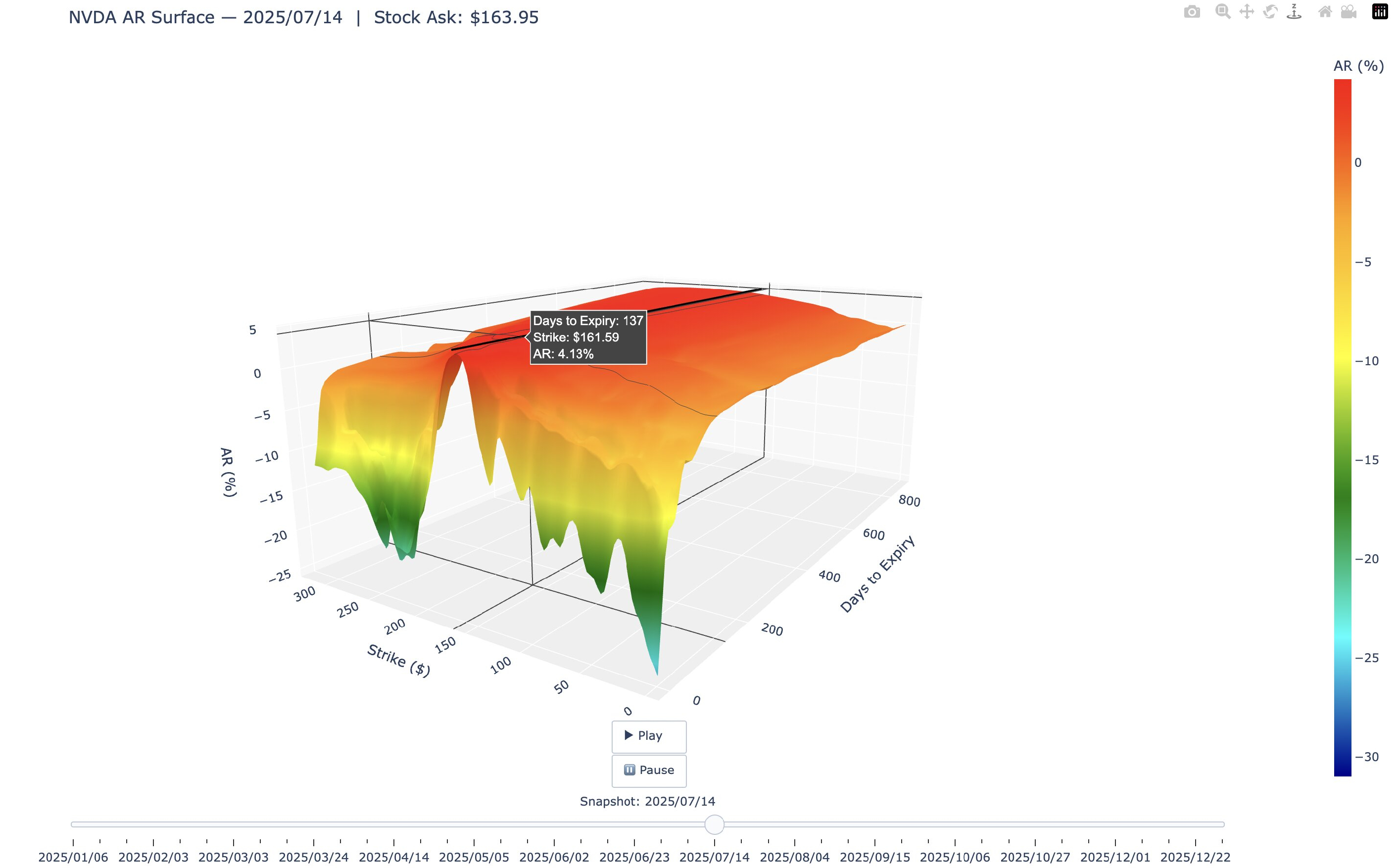
NVDA annualized-return surface on July 14, 2025, showing the highest annualized returns along the near-the-money ridge.

The image shows the annualized-return surface for NVDA on a single day. Near-the-money, short-dated strikes consistently dominate the surface because the same dollar premium annualizes to a higher return over a shorter time horizon. The strategy scans this surface across all seven stocks each morning and selects the global maximum.

Dynamic Contract Swapping

Holding the best conversion at entry is not the end of the story because an opportunity with a greater annualized return can appear while the position is open. At each scan, the algorithm compares a candidate trade's annualized return against the return of the position that's already in the portfolio. It swaps only when the candidate's annualized return exceeds the sum of the open position's return, the cost of unwinding its legs, and a fixed hurdle,

\[ \text{AR}_\text{market} > \text{AR}_\text{hand} + \text{AR}_\text{exit} + h, \]

where \( \text{AR}_\text{market} \) and \( \text{AR}_\text{hand} \) are the candidate's and the open position's annualized returns, \( \text{AR}_\text{exit} \) is the round-trip bid-ask cost of closing the position, and \( h \) is the hurdle. The hurdle keeps the strategy from churning through marginally better trades and paying away the edge in transaction costs.

Implementation

To implement this strategy, we start by adding the Magnificent 7 Equities, their Option chains, and a Treasury ETF to hold idle cash.

self._shv = self.add_equity('SHV')
tickers = ["AAPL", "MSFT", "NVDA", "AMZN", "META", "GOOGL", "TSLA"]  # Mag 7 stocks only
self._equities = []
for ticker in tickers:
    equity = self.add_equity(ticker)
    option = self.add_option(ticker)
    option.set_filter(lambda u: u.include_weeklys().expiration(7, 36).strikes(-30, 0))
    equity.option_symbol = option.symbol
    self._equities.append(equity)

The trading logic only takes conversions with a positive net premium, so the Option universe filter only selects strikes below the underlying price, where the call is worth more than the put. It also limits the universe to contracts expiring in 7 to 36 days.

The strategy opens a conversion only when its annualized return clears a 5% minimum. Swapping is a distinct test that requires the candidate to beat the open position's return by the cost of switching plus a 3% margin. A Scheduled Event runs the _check_for_entry method every 5 minutes over the first 30 minutes after the open, when the quotes are most active. The first scan fires one minute after the open rather than at the open itself, so it acts on the day's first quotes rather than the previous close. A separate Scheduled Event liquidates any position on its expiry day.

self._min_ar = 5  # Minimum AR threshold to buy contract
self._swap_optimization = 3 # Minimum AR improvement required to justify a swap
for i in range(7):
    self.schedule.on(
        self.date_rules.every_day('SPY'),
        self.time_rules.after_market_open('SPY', max(5*i, 1)), 
        self._check_for_entry
    )

Each time _check_for_entry runs, it calls the _find_best_trade helper method to find the best opportunity across the universe. The _find_best_trade method first scans each stock's Option chain and groups the contracts into call-put pairs that share a strike and expiry.

chain = self.current_slice.option_chains.get(underlying.option_symbol)
if not chain:
    continue
pairs = defaultdict(dict)
for contract in chain:
    key = (contract.strike, contract.expiry.date())
    pairs[key][contract.right] = contract

For each pair, it keeps conversions with a positive net premium, tradable call and put quotes, and a strike within 10% of the underlying price, then records the candidate's annualized return. The method returns the single pair with the highest annualized return.

for (strike, expiry), legs in pairs.items():
    call = legs.get(OptionRight.CALL)
    put = legs.get(OptionRight.PUT)
    if not call or not put:
        continue
    s = strike
    c = call.bid_price
    p = put.ask_price
    net_premium = c - p
    if (net_premium < 0 or 
        c <= 0 or p <= 0 or 
        s < 0.90 * underlying_price or s > 1.10 * underlying_price):
        continue

The _annualized_return helper method values each conversion at executable prices, the call bid, the put ask, and the stock ask, so the value reflects what the trade actually captures after crossing the spread.

def _annualized_return(self, underlying, call, put):
    c = self.securities[call.symbol].bid_price 
    p = self.securities[put.symbol].ask_price
    a = underlying.ask_price
    s = call.strike
    t = self._years_to_expiry(call.expiry.date())
    return ((c - p) + (s - a)) * 100 / (a * t)

With that best candidate in hand, _check_for_entry decides what to do. When an open conversion reaches expiry or loses its stock leg to early assignment, it closes the position. Otherwise, it swaps into the best candidate only when that candidate's annualized return exceeds the the open position's return, the exit cost, and the swap hurdle

if self._trade:
    if (self.time.date() >= self._trade.expiry or
        not self._trade.underlying.invested and self.time.date() < self._trade.expiry):
        self.liquidate()
        self._trade = None
    elif best_trade and best_trade["ar"] > self._get_hand_ar() + self._get_exit_cost() + self._swap_optimization:
        self.liquidate()
        self._trade = None
        self._enter_position(best_trade)

The _enter_position helper method sizes the trade to roughly 95% of available margin and submits a single combo market order that buys the stock, buys the put, and sells the call together.

combo_price = 100 * (underlying.ask_price + put.ask_price - call.bid_price)
combos = int(self.portfolio.margin_remaining * .95 / combo_price)
if combos < 1:
    return
legs = [
    Leg.create(underlying, 100),
    Leg.create(put.symbol, 1),
    Leg.create(call.symbol, -1)
]
self.combo_market_order(legs, combos)

Results

We backtested the strategy from January 2023 to June 2026. The strategy produced a −0.08 Sharpe ratio. In contrast, a buy-and-hold position in the SPY earned a 0.902 Sharpe ratio over the same period. Therefore, the strategy underperforms the benchmark in terms of risk-adjusted returns once you factor in the risk-free rate.

We ran a parameter optimization job to test the sensitivity of the chosen parameters. We tested a minimum annualized return from 3% to 8% in steps of 1%, and we tested the number of 5-minute entry scans after the open from 4 to 10 in steps of 1. Of the 42 parameter combinations, 0/42 (0%) produced a greater Sharpe ratio than the benchmark. The following image shows the heatmap of Sharpe ratios for the parameter combinations:

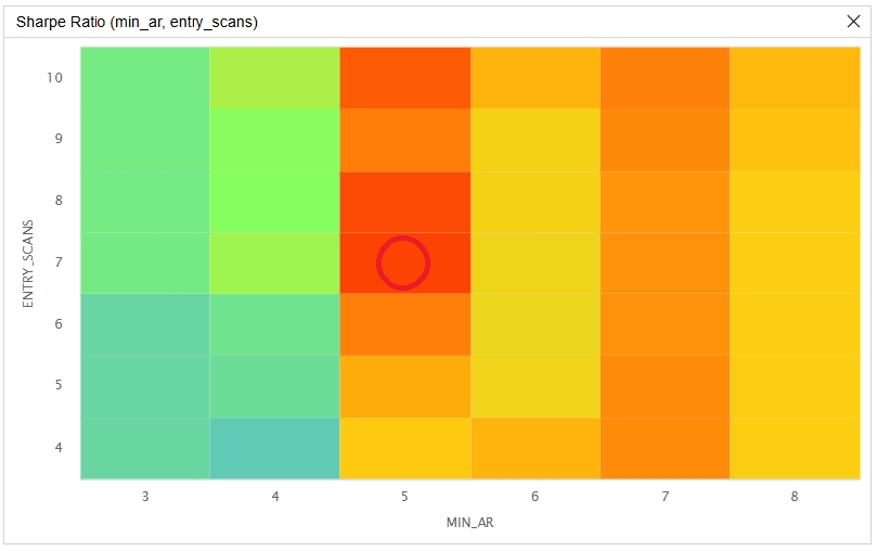
The red circle in the preceding image identifies the parameters we chose as the strategy's default. We chose a minimum annualized return of 5% and 7 entry scans because that combination produced the highest Sharpe ratio in the grid.

The minimum annualized return is the parameter that matters. The Sharpe ratio peaks at a 5% threshold and falls away for both looser and stricter minimums. The number of entry scans is the less influential parameter and the surface is nearly flat along it, so scanning later into the morning neither materially helps nor hurts.

The strategy produces a negative Sharpe ratio because of the risk-free rate. However, reviewing the strategy's other performance measures provides clear insight into the strategy's performance without the risk-free rate dominating the results. With the default parameter values, the strategy earned a 7.5% compounding annual return, a 1.1% maximum drawdown, a 2.7% annualized volatility, and a 0.017 beta. The 1.1% drawdown is a fraction of the SPY's 18.8% over the same period, so the strategy reached its return with far less risk than the market.

Overall, the strategy turns a textbook arbitrage into a low-drawdown return stream, and it stays profitable across the entire parameter grid rather than at a single setting. Natural extensions are to optimize the swap hurdle and to widen the universe beyond the Magnificent 7.

References

• Stoll, H. R. (1969). The relationship between put and call option prices. Journal of Finance, 24(5), 801–824.