Futures Trend Following and Carry in Different Risk Regimes

Introduction

In this tutorial, we build upon the Combined Carry and Trend strategy to include dynamic position sizing based on the current risk regime. When the relative level of risk is lower than normal, we take larger positions and when it’s higher than normal, we take smaller positions. The results show that adjusting the position sizing based on the current risk regime significantly increases the risk-adjusted returns of the strategy. This algorithm is a re-creation of strategy #13 from Advanced Futures Trading Strategies (Carver, 2023).

Quantifying Risk Regimes

Let \(r\) be a series of daily returns for a continuous contract. Using a span of \(\lambda\), the exponentially-weighted moving average of \(r\) is

\[r^*(\lambda)_t = \lambda r_t + \lambda(1-\lambda)r_{t-1} + \lambda(1-\lambda)^2 r_{t-2} + . . .\]

and the exponentially-weighted standard deviation of \(r\) is 

\[\sigma_{exp}(\lambda)_t = \sqrt{ \lambda(r_t - r^*_t)^2 + \lambda(1-\lambda)(r_{t-1} - r^*_t)^2 + \lambda(1-\lambda)^2(r_{t-2}-r^*_t)^2 + ... }\]

If we assume there are 256 trading days in a year, the annualized exponentially-weighted standard deviation of \(r\) is 

\[\sigma_{ann}(\lambda)_t = \sigma_{exp}(\lambda)_t \times \sqrt{256}\]

Volatility tends to cluster in the short run and mean revert in the long run. To improve the forecasts and reduce the possibility of entering large positions before a crisis, we can blend together a long run and short run estimate of volatility.

\[\sigma_{\%,t} = 0.3(\textrm{Ten year average of }\sigma_{ann}(\lambda)_t) + 0.7\sigma_{ann}(\lambda)_t\]

The relative level of volatility is then

\[V_{t} = \frac{\sigma_{\%,t}}{ \textrm{Ten year average of } \sigma_{\%,t}}\]

The quantile point \(Q_{t}\) of the relative level of volatility \(V_{t}\) is

\[Q_t = \textrm{Quantile of }V_t\textrm{ in distribution}(V_0, ..., V_t) \in [0, 1]\]

The way this works is 

\[V_t = min(V) \implies Q_t = 0\]
\[V_t = max(V) \implies Q_t = 1\]

Given \(Q_{t}\), the volatility multiplier \(M_{t}\) is

\[M_t = EWMA_{\textrm{span}=10}(2 - 1.5 \times Q_t) \in [0.5, 2]\]

\(M_{t}\) acts as the volatility multiplier because when volatility is very low (\(Q_{t} = 0\)), \(M_{t} = 2\). When volatility is very high (\(Q_{t} = 1\)), \(M_{t} = 0.5\). In the next couple sections, we’ll use \(M_{t}\) to scale our forecasts.

Risk-Adjusted Trend Forecasts

The Combined Carry and Trend strategy used 3 trend filters to produce forecasts. In this strategy, we'll use the same ones. The process of calculating the trend forecast is similar to the previous iteration of the strategy, except we scale the forecast by the volatility multiplier.

\[\textrm{Raw forecast} = \frac{EMAC(n,4n)}{\sigma_{\%,t}}\]
\[\textrm{Scaled forecast} = \textrm{Raw forecast} \times M_t \times \textrm{Forecast scalar}\]
\[\textrm{Capped forecast} = \max(\min(\textrm{Scaled forecast}, 20), -20)\]

The following table shows the forecast scalars provided by Carver for each EMAC span. These values are the same as the ones in the Combined Carry and Trend strategy.

Risk-Adjusted Carry Forecasts

The process of calculating the carry forecast is similar to the Combined Carry and Trend strategy, except we scale the forecast by the volatility multiplier and we change the forecast scalar.

\[\textrm{Smoothed carry (span) forecast} = EWMA_\textrm{span}(\textrm{carry forecast})\]
\[\textrm{Adjusted smoothed carry (span) forecast} = \textrm{Smoothed carry (span) forecast} \times M_t \times \textrm{Forecast scalar}\]
\[\textrm{Capped forecast} = \textrm{max(min}(\textrm{Adjusted smoothed carry (span) forecast}, 20), -20)\]

The forecast multiplier again scales the forecast to have an average absolute value of 10. Carver provides the forecast scalar to use, which is 23. 

Aggregating Forecasts

Each day, we have several risk-adjusted trend forecasts and several risk-adjusted carry forecasts. The trend component of this strategy is a divergent factor and the carry component is a convergent factor. To aggregate all these forecasts together, we use the same methodology as the Combined Carry and Trend strategy:

1. Calculate the mean trend forecast.
2. Calculate the mean carry forecast.
3. Mix the means together by giving a 60% weight to the mean trend forecast and a 40% weight to the mean carry forecast.
4. Apply a forecast diversification multiplier to keep the average aggregated forecast at a value of 10.
5. Cap the result to be within the interval [-20, 20].

Method

Let’s walk through how we can implement this trading algorithm with the LEAN trading engine. Most of the code is the same as the previous Futures strategies we’ve seen, so let’s just review the changes.

Universe Selection

We keep the same universe from the Combined Carry and Trend strategy, which contains a diversified set of 19 Futures.

Risk Regime Multiplier

To calculate the relative level of volatility \(V_{t}\), adjust the estimate_std_of_pct_returns method in the alpha.py file to return a series of blended estimates.

def estimate_std_of_pct_returns(self, raw_history, adjusted_history):
    # Align history of raw and adjusted prices
    raw_history_aligned, adjusted_history_aligned = self.align_history(raw_history, adjusted_history)

    # Calculate exponentially weighted standard deviation of returns
    returns = adjusted_history_aligned.diff().dropna() / raw_history_aligned.shift(1).dropna() 
    rolling_ewmstd_pct_returns = returns.ewm(span=self.sigma_span, min_periods=self.sigma_span).std().dropna()
    if rolling_ewmstd_pct_returns.empty: # Not enough history
        return None
    # Annualize sigma estimate
    annulized_rolling_ewmstd_pct_returns = rolling_ewmstd_pct_returns * (self.annulaization_factor)
    # Blend the sigma estimate (p.80, p.260)
    historical_averages = annulized_rolling_ewmstd_pct_returns.rolling(2*self.blend_years*self.BUSINESS_DAYS_IN_YEAR).mean().dropna()
    blended_estimates = 0.3*historical_averages + 0.7*annulized_rolling_ewmstd_pct_returns.iloc[-len(historical_averages):]
    return blended_estimates

To calculate the quantile point \(Q_{t}\) of any series, add the following helper method to the Alpha model:

def quantile_of_points_in_data_series(self, data_series):
    ## With thanks to https://github.com/PurpleHazeIan for this implementation
    numpy_series = np.array(data_series)
    results = []

    for irow in range(len(data_series)):
        current_value = numpy_series[irow]
        count_less_than = (numpy_series < current_value)[:irow].sum()
        results.append(count_less_than / (irow + 1))

    results_series = pd.Series(results, index=data_series.index)
    return results_series

With the helper method defined, add the following method to calculate the volatility multiplier \(M_{t}\):

def get_vol_regime_multiplier(self, sigma_pcts):
    # Calculate volatility quantile
    sigma_pct_averages = sigma_pcts.rolling(self.blend_years*self.BUSINESS_DAYS_IN_YEAR).mean().dropna()
    normalized_vol = sigma_pcts.iloc[-len(sigma_pct_averages):] / sigma_pct_averages
    normalized_vol_q = self.quantile_of_points_in_data_series(normalized_vol)
    # Calculate volatility regime multiplier
    vol_attenuation = 2 - 1.5*normalized_vol_q
    return vol_attenuation.ewm(span=10).mean().dropna().iloc[-1]

Now that you have \(M_{t}\), pass it to the forecasting methods.

Risk-Adjusted Trend Forecasts

The method to calculate the EMAC forecasts is similar to previous Futures strategies, but it now includes the volatility multiplier.

def emac_adjusted_for_vol_regime(self, ewmac_by_span, daily_risk_price_terms, vol_regime_multiplier):
    forecasts = []
    for span in self.emac_spans:
        risk_adjusted_ewmac = ewmac_by_span[span].Current.Value / daily_risk_price_terms                
        risk_adjusted_ewmac *= vol_regime_multiplier
        scaled_forecast_for_ewmac = risk_adjusted_ewmac * self.TREND_FORECAST_SCALAR_BY_SPAN[span]
        capped_forecast_for_ewmac = max(min(scaled_forecast_for_ewmac, self.abs_forecast_cap), -self.abs_forecast_cap)
        forecasts.append(capped_forecast_for_ewmac)
    return forecasts

Risk-Adjusted Carry Forecasts

The method to calculate the carry forecasts is similar to the Combined Carry and Trend strategy, but it now includes the volatility multiplier.

def carry_adjusted_for_vol_regime(self, annualized_raw_carry, daily_risk_price_terms, vol_regime_multiplier):
    carry_forecast = annualized_raw_carry / daily_risk_price_terms

    forecasts = []
    for span in self.carry_spans:
        ## Smooth out carry forecast
        smoothed_carry_forecast = carry_forecast.ewm(span=span, min_periods=span).mean().dropna()
        if smoothed_carry_forecast.empty:
            continue
        smoothed_carry_forecast = smoothed_carry_forecast.iloc[-1]
        ## Adjust forecast based on volatility regime (p. 263)
        adjusted_smoothed_carry_forecast = smoothed_carry_forecast * vol_regime_multiplier  
        ## Apply forecast scalar (p. 264)
        scaled_carry_forecast = adjusted_smoothed_carry_forecast * self.CARRY_FORECAST_SCALAR
        ## Cap forecast
        capped_carry_forecast = max(min(scaled_carry_forecast, self.abs_forecast_cap), -self.abs_forecast_cap)
        forecasts.append(capped_carry_forecast)
    return forecasts

Aggregating Forecasts

The following changes to the Update method summarizes how we aggregate all of the forecasts into a single value:

def Update(self, algorithm: QCAlgorithm, data: Slice) -> List[Insight]:        
    # . . . 
    for symbol, instrument_weight in weight_by_symbol.items():
        # Calculate volatility regime multiplier
        vol_regime_multiplier = self.get_vol_regime_multiplier(sigma_pcts_by_future[future])

        # Calculate forecast type 1: EMAC adjusted for volatility regime
        trend_forecasts = self.emac_adjusted_for_vol_regime(future.ewmac_by_span, daily_risk_price_terms, vol_regime_multiplier)
        if not trend_forecasts:
            continue
        emac_combined_forecasts = sum(trend_forecasts) / len(trend_forecasts) # Aggregate EMAC factors -- equal-weight

        # Calculate factor type 2: Carry adjusted for volatility regime
        carry_forecasts = self.carry_adjusted_for_vol_regime(future.annualized_raw_carry_history, daily_risk_price_terms, vol_regime_multiplier)
        if not carry_forecasts:
            continue
        carry_combined_forecasts = sum(carry_forecasts) / len(carry_forecasts) # Aggregate Carry factors -- equal-weight
        
        # Aggregate factors -- 60% for trend, 40% for carry
        raw_combined_forecast = 0.6 * emac_combined_forecasts + 0.4 * carry_combined_forecasts
        scaled_combined_forecast = raw_combined_forecast * self.FDM_BY_RULE_COUNT[len(trend_forecasts) + len(carry_forecasts)] # Apply a forecast diversification multiplier to keep the average forecast at 10 (p 193-194)
        capped_combined_forecast = max(min(scaled_combined_forecast, self.abs_forecast_cap), -self.abs_forecast_cap)
    # . . . 

Calculating Position Sizes

This algorithm uses the same trade buffering logic as the Combined Carry and Trend strategy.

Results

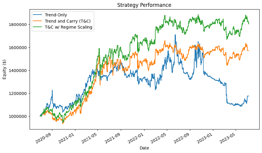
We backtested the strategy from July 1, 2020 to July 1, 2023. The algorithm achieved a 0.944 Sharpe ratio. In contrast, the Combined Carry and Trend strategy achieved a 0.749 Sharpe ratio. Therefore, adjusting the strategy’s position sizes by the volatility multiplier significantly increases the risk-adjusted returns of the strategy. The following chart shows the equity curves of the Fast Trend Following strategy, the Combined Carry and Trend strategy, and strategy outlined in this research post:

Further Research

If you want to continue developing this strategy, some areas of further research include:

• Tracking the performance of each factor and removing the ones that are too expensive to trade
• Incorporating other convergent/divergent factors
• Calculating the forecast diversification multiplier on the fly instead of using the hard-coded estimates provided above

References

1. Carver, R. (2023). Advanced Futures Trading Strategies: 30 fully tested strategies for multiple trading styles and time frames. Harriman House Ltd.