


Introduction
The MAX effect describes how stocks with extreme positive daily returns behave like lotteries and subsequently underperform, so the calmer names left behind earn higher risk-adjusted returns. In this research, we test this anomaly on US Equities and add a volatility overlay that scales portfolio leverage with the CBOE Volatility Index (VIX). Each month, we rank the liquid US Equity universe by a MAX factor and hold an equal-weighted portfolio of the lowest-MAX decile, then lever the book up to 1.5x when the VIX is calm and back to 1x when it spikes. Since 1998, the strategy earned a 0.57 Sharpe ratio, outperforming the 0.335 Sharpe ratio of a buy-and-hold position in SPY over the same period.
Background
Bali, Cakici, and Whitelaw (2011) showed that investors overpay for stocks with lottery-like payoffs. Sorting US Equities on the average of their highest daily returns over the prior month, they found the highest-MAX stocks went on to badly underperform the lowest-MAX stocks, even after controlling for size, value, momentum, and short-term reversal factors. The intuition is behavioral. Some investors hold a preference for positive skewness and bid up stocks that recently experiences a few spectacular up-days, which leaves those stocks overpriced and the calmer stocks underpriced.
We harvest this premium from the long side. Each month, we buy the Equities in the bottom decile of the MAX factor and hold them equally-weighted, which avoids the crash risk of shorting the high-MAX leg. We then overlay a volatility-timing rule that adds leverage in calm regimes and removes it in turbulent ones.
The MAX Factor
For each stock, we compute the MAX factor as the mean of its five largest daily returns over the trailing 21 trading days.
\[ \text{MAX}^{(5)}_{i} = \frac{1}{5} \sum_{k=1}^{5} R_{i,(k)} \]
Here \( R_{i,(k)} \) is the \( k \)-th largest daily return of stock \( i \) over the trailing month. Averaging the top five returns rather than the single maximum produces a less noisy estimate of a stock's lottery character. A low \( \text{MAX}^{(5)} \) marks a stock that has lacked recent extreme up-days, which is exactly the profile the anomaly rewards.
VIX-Responsive Leverage
The VIX measures the market's expectation of 30-day volatility implied by S&P 500 Index Option prices, so a low VIX signals a calm regime and a high VIX a fearful one. We treat the VIX as a regime switch and set portfolio leverage as a piecewise-linear function of its level.
\[L(\text{VIX}) =\begin{cases}1.5, & \text{VIX} \le 15 \\[4pt]1.5 - \dfrac{\text{VIX} - 15}{15}\times 0.5, & 15 < \text{VIX} < 30 \\[4pt]1.0, & \text{VIX} \ge 30\end{cases}\]
When implied volatility is low, we increase leverage to 1.5x. As fear rises toward a VIX of 30, we decrease leverage back to 1x. This keeps the most aggressive sizing for the quiet periods in which the anomaly tends to compound steadily, while cutting risk into the volatility spikes that drive the strategy's deepest drawdowns.
Implementation
To implement this strategy, we start by adding a US Equity fundamental universe, adding the VIX, and scheduling the monthly rebalance in the initialize method.
self._universe = self.add_universe(self._select_assets)
self._vix = self.add_data(CBOE, 'VIX', Resolution.DAILY)
self._low_vix = 15
self._high_vix = 30
self.schedule.on(self.date_rules.month_start('SPY', 1), self.time_rules.at(8, 0), self._rebalance)
The Scheduled Event fires on the first trading day of each month at 8 AM Eastern Time (ET). In live trading, universe selection runs between 7 AM and 8 AM ET, so firing at 8 AM ensures the rebalance sees the current day's universe.
In the selection function, we select stocks priced above $5 per share with a market capitalization above $1 billion.
for f in fundamentals:
    # Apply universe filters.
    if (f.company_reference.is_reit or
        f.security_reference.is_depositary_receipt or
        not f.has_fundamental_data or
        f.price < 5 or
        f.market_cap < 1_000_000_000):
        continue
For each stock in the universe, the algorithm maintains a SelectionData object, which tracks the daily returns and average daily dollar volume of the stock over the trailing month.
self.dollar_volume_sma = SimpleMovingAverage(period)
self._daily_return = RateOfChange(1)
self._daily_return.window.size = period
On each universe selection, it updates both indicators with the stock's latest values.
def update(self, f: Fundamental) -> bool:
    self.dollar_volume_sma.update(f.end_time, f.dollar_volume)
    self._daily_return.update(f.end_time, f.adjusted_price)
    return self.is_ready
The MAX factor is then the mean of the stock's five largest daily returns over the month.
@property
def factor(self) -> float:
    # Get the mean of the top n trailing daily returns.
    return float(np.mean(sorted([x.value for x in self._daily_return.window])[-self._top_returns:]))
At each rebalance, we read the current universe constituents and collect the MAX factor for every stock whose 21-day average dollar volume is at least $5 million.
securities = [self.securities[symbol] for symbol in self._universe.selected]
factor_by_security = {}
for security in securities:
    data = self._selection_data_by_symbol[security.symbol]
    if security.price and data.dollar_volume_sma.current.value >= 5_000_000:
        factor_by_security[security] = data.factor
We then rank by the factor and buy the bottom decile (capped at 25 stocks) and equally-weight them.
sorted_by_factor = sorted(factor_by_security, key=lambda security: factor_by_security[security])
selection_size = min(25, len(sorted_by_factor) // 10)
securities = sorted_by_factor[:selection_size]
weight = 1 / len(securities)
self._trade({security: weight for security in securities})
The _trade method sizes the positions with the VIX-responsive leverage rule, increasing exposure to 1.5x when the VIX is at or below 15 and decreasing to 1x as it rises toward 30.
vix = self._vix.price
if not vix or vix >= self._high_vix:
    leverage = 1.0
elif vix <= self._low_vix:
    leverage = 1.5
else:
    leverage = 1.5 - (vix - self._low_vix) / self._low_vix * 0.5
The algorithm scales the target weights by this leverage and submits them as portfolio targets.
# Scale portfolio weights based on target portfolio exposure.
targets = [PortfolioTarget(s, leverage * w ) for s, w in weight_by_security.items()]
self.set_holdings(targets, liquidate_existing_holdings=True)
Between the monthly rebalances, the algorithm continues to monitor the VIX and adjusts the portfolio's leverage whenever it crosses 15 or 30, scaling every position by the same factor so the relative weights between positions don't change.
Results
We backtested the algorithm from January 1998 to June 2026. Over that period, the strategy earned a 0.57 Sharpe ratio. In contrast, a buy-and-hold position in the SPY over the same time period achieved a 0.335 Sharpe ratio. Therefore, the strategy outperformed the benchmark.
We ran a parameter optimization job to test the sensitivity of the chosen parameters. We tested the number of top daily returns averaged into the MAX factor (top_returns) from 3 to 7 in steps of 1, and the number of stocks held in the portfolio (max_portfolio_size) from 15 to 35 in steps of 5. Of the 25 parameter combinations, 25/25 (100%) produced a greater Sharpe ratio than the benchmark. The following image shows the heatmap of Sharpe ratios for the parameter combinations:
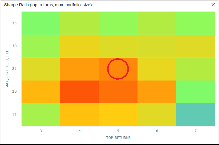
The red circle in the preceding image identifies the parameters we chose as the strategy's default. We chose a top_returns value of 5 and a max_portfolio_size of 25 because a value of 5 matches the five-return MAX measure defined in the source paper, and a 25-stock portfolio sits inside the flat, high-Sharpe region near the optimizer's peak.
The surface is shallow. Across all 25 combinations the Sharpe ratio stays within a narrow band, from 0.474 to 0.585, so neither parameter is fragile. The number of returns averaged into the factor is the most sensitive parameter. The Sharpe ratio is strongest when it averages four or five returns and falls off as that count rises toward seven. The portfolio size matters less. A 20-stock portfolio is the best across most rows. A larger portfolio reduces the Sharpe as it dilutes the lowest-MAX names. Both best values sit inside the tested ranges rather than at an edge of the grid search, so widening the search is unlikely to improve the results.
In conclusion, every parameter combination we tested beat the buy-and-hold benchmark in terms of risk-adjusted returns and the strong region is broad rather than a single lucky cell, which suggests the MAX effect itself drives the result. Future research could add a short leg in the highest-MAX names to neutralize market exposure, or replace the static VIX thresholds with a percentile-based regime measure.
References
- Bali, T. G., Cakici, N., & Whitelaw, R. F. (2011). Maxing out: Stocks as lotteries and the cross-section of expected returns. Journal of Financial Economics, 99(2), 427–446. https://www.sciencedirect.com/science/article/abs/pii/S0304405X1000190X


Derek Melchin
The material on this website is provided for informational purposes only and does not constitute an offer to sell, a solicitation to buy, or a recommendation or endorsement for any security or strategy, nor does it constitute an offer to provide investment advisory services by QuantConnect. In addition, the material offers no opinion with respect to the suitability of any security or specific investment. QuantConnect makes no guarantees as to the accuracy or completeness of the views expressed in the website. The views are subject to change, and may have become unreliable for various reasons, including changes in market conditions or economic circumstances. All investments involve risk, including loss of principal. You should consult with an investment professional before making any investment decisions.
To unlock posting to the community forums please complete at least 30% of Boot Camp.
You can continue your Boot Camp training progress from the terminal. We hope to see you in the community soon!