Filing Language Stability as a Selection Signal

Research conducted by: Emily Xinyu Sun - Mentored by Rudy Osuna - Triton Quantitative Trading @ UC San Diego

Introduction

Every public company files a 10-K with the SEC each year and a 10-Q after each of its first three quarters. These are the audited annual report and the lighter quarterly updates that disclose a firm's financial results and business risks. They draw investor attention to the reported numbers, yet the language of the filing carries information of its own. Cohen, Malloy, and Nguyen (2020) document that firms which barely change their filing language from one year to the next earn higher subsequent returns than firms that substantially rewrite their disclosures, an effect they call Lazy Prices. We turn this finding into a long-only stock-selection strategy on the 100 most liquid US Equities. Each month we rank them on the language similarity of their latest 10-K and 10-Q filings, drawn from the Brain Language Metrics on Company Filings dataset, and hold a long-only portfolio of the most stable filers, weighted to maximize the portfolio Sharpe ratio. From January 2020 to June 2026, the strategy produced greater risk-adjusted returns than the benchmark SPY ETF.

Background 

A 10-K or 10-Q is mostly boilerplate that management carries forward from the previous period with minor edits. Cohen, Malloy, and Nguyen study what happens in the unusual cases when a firm materially rewrites that language, especially the risk-factors and management-discussion sections. They find that these changes are a strong negative signal for future returns. Firms that change their disclosures, the "changers", go on to earn lower returns, while firms that leave them stable, the "non-changers", earn higher returns. The changes also predict future earnings, news, and even bankruptcies, yet there is no price reaction at the filing date.

The label "lazy prices" captures the mispricing. Prices are slow to incorporate the information embedded in the presence or absence of textual change, because reading two filings side by side is tedious and few investors do it. We measure filing stability with a textual similarity score, a number between zero and one that captures how much of a filing's language is carried over from the company's previous comparable filing. A score near one marks a filing that closely repeats its predecessor, while a lower score marks one that has been heavily rewritten. 

We read these scores from the Brain Language Metrics on Company Filings dataset, which reports a full-report score and a risk-factors-section score for every 10-K and 10-Q. The strategy ranks the 100 most liquid US Equities on this similarity each month and treats the most similar filers as the most stable, the side of the signal the Lazy Prices effect rewards. We prefer the risk-factors similarity, the section the paper finds most informative, and we fall back to the full-report similarity when the first is unavailable. Ranking the universe by this score and keeping the top stocks selects the laziest, most stable filers.

Rather than weight the selected stocks equally, we size them to maximize the portfolio's historical Sharpe ratio. The optimizer searches for the weight vector that maximizes

\[ \frac{w^\top \mu}{\sqrt{w^\top \Sigma w}}\]
where \(w\) is the vector of portfolio weights, \(\mu\) is the vector of mean daily returns over the lookback window, and \( \Sigma\) is the covariance matrix of those returns. We constrain the weights to the interval \([0, 1]\), which forces a long-only portfolio that is fully invested across the selected stocks. The lookback window that supplies \(\mu\) and \(\Sigma\) is set to twelve months of daily returns by default.

Implementation

To implement this strategy, we start by setting the data resolution and scheduling universe selection to run on the first trading day of each month, matching the rebalance cadence. The algorithm adds two universes. A fundamental universe narrows the market to the most liquid stocks, and the Brain filing universe then ranks textual similarity within that set.

self.universe_settings.resolution = Resolution.DAILY
self._date_rule = self.date_rules.month_start("SPY")
self.universe_settings.schedule.on(self._date_rule)
self.add_universe(self._fundamental_filter)
self._universe = self.add_universe(BrainCompanyFilingLanguageMetricsUniverseAll, self._select_assets)

During initialization we also create the Sharpe optimizer, giving it a lookback window of twelve months, which supplies a full year of daily returns.

self._optimizer = SharpePortfolioOptimizer()

The _fundamental_filter method stores the 100 stocks with the highest average dollar volume that have fundamental data. It returns an unchanged universe and only caches these symbols, so the Brain filing universe can later rank within this liquid set.

def _fundamental_filter(self, fundamentals: List[Fundamental]) -> Universe.UnchangedUniverse:
    # Store the 100 most liquid Equities; the Brain filing universe ranks within this set.
    self._fundamentals = [f.symbol for f in sorted([f for f in fundamentals if f.has_fundamental_data], key=lambda f: f.dollar_volume)[-100:]]
    return Universe.UNCHANGED

The _select_assets method reads six months of filing history from the BrainCompanyFilingLanguageMetricsUniverseAll universe, keeps only the stocks that survived the liquidity filter, and records each one's most recent similarity score, preferring the risk-factors similarity over the full-report similarity.

def _select_assets(self, filings: List[BrainCompanyFilingLanguageMetricsUniverseAll]) -> List[Symbol]:
    similarity_by_symbol = {}
    # Scan the past 6 months of 10-K/10-Q filings for similarity scores.
    history = self.history(self._universe, timedelta(30 * 6), Resolution.DAILY)
    for daily_filings in history:
        for filing in daily_filings:
            if filing.symbol not in self._fundamentals:
                continue
            # Prefer risk factors similarity scores, else the full report similarity scores.
            similarity = filing.risk_factors_statement_sentiment.similarity.all or filing.report_sentiment.similarity.all
            if similarity:
                similarity_by_symbol[filing.symbol] = similarity

It then returns the top 25 stocks by highest similarity.

return sorted(similarity_by_symbol, key=lambda symbol: similarity_by_symbol[symbol])[-25:]

A Scheduled Event fires the _rebalance method at 8 AM Eastern Time (ET) on the first trading day of each month, the same monthly rule that drives universe selection.

time_rule = self.time_rules.at(8, 0)
self.schedule.on(self._date_rule, time_rule, self._rebalance)

The _rebalance method passes the current universe constituents to the SharpePortfolioOptimizer, builds a portfolio target for each returned weight, and rebalances to those weights while liquidating any holdings that left the selection.

weight_by_symbol = self._optimizer.get_weights(self, list(self._universe.selected))
targets = [PortfolioTarget(symbol, weight) for symbol, weight in weight_by_symbol.items()]
self.set_holdings(targets, True)

The get_weights method does the sizing. It requests daily closes over a 12 month lookback window with a history request, converts them to daily returns, and calls LEAN's MaximumSharpeRatioPortfolioOptimizer to produce the long-only weights.

def get_weights(self, algorithm: QCAlgorithm, symbols: list) -> dict:
    history = algorithm.history(symbols, self._period + 1, Resolution.DAILY)
    returns = history["close"].unstack(level=0).pct_change().dropna()
    # Maximize the portfolio Sharpe ratio using the long-only optimizer.
    raw_weights = self._optimizer.optimize(returns)
    return {symbol: float(raw_weights[i]) for i, symbol in enumerate(returns.columns)}

Results

We backtested the strategy from January 2020 to June 2026. Over that period the strategy earned a 0.558 Sharpe ratio. In contrast, a buy-and-hold position in the SPY over the same time period achieved a 0.533 Sharpe ratio [Backtest link]. Therefore, the strategy outperformed the benchmark.

We ran a parameter optimization job to test the sensitivity of the chosen parameters. We tested lookback_months, the number of months of return history the optimizer uses to size positions, from 6 to 30 months in steps of 6. We also tested universe_size, the number of stocks held, from 10 to 30 in steps of 5. Of the 25 parameter combinations, 9 of 25 (36%) produced a greater Sharpe ratio than the benchmark. The following image shows the heatmap of Sharpe ratios for the parameter combinations:

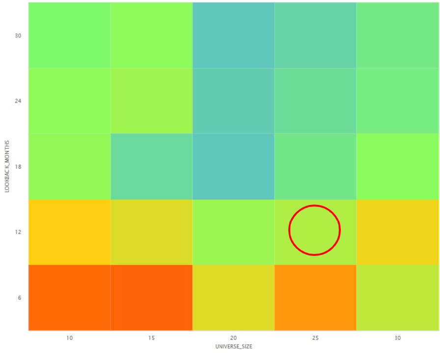
The red circle in the image above identifies the parameters we chose as the strategy's default. We chose a lookback_months of 12 because a full year of daily returns gives the optimizer a more robust covariance estimate than a shorter window. We chose a universe_size of 25 because a broader basket spreads risk across more stocks and reduces concentration risk. The sensitivity analysis shows the result is driven mainly by the optimizer's lookback window rather than the breadth of the basket, and that shorter windows scored higher in sample. Future research could add the short leg of the Lazy Prices anomaly, selling the firms that most rewrote their filings, moving the strategy toward the original long-short design. That extension naturally invites different optimizer constraints, such as dollar neutrality, to balance the long and short books.

Conclusion

This research turns the Lazy Prices effect into a simple, tradeable strategy. Each month it ranks the 100 most liquid US Equities on the language stability of their latest 10-K and 10-Q filings, drawn from the Brain Language Metrics on Company Filings dataset, and holds the most stable filers in a long-only portfolio weighted to maximize the Sharpe ratio. From January 2020 to June 2026 the strategy produced a 0.558 Sharpe ratio, outperforming a buy-and-hold position in the SPY. The result shows that disclosure-language stability carries tradable information beyond a firm's reported numbers, though the strategy's edge depends on the quality of the filing-similarity scores and warrants further testing across market regimes.

References

Cohen, Lauren, et al. “Lazy Prices.” The Journal of Finance, vol. 75, no. 3, 22 Feb. 2020, pp. 1371–1415, https://doi.org/10.1111/jofi.12885.