


 Share New Research


Introduction
The volatility risk premium is the tendency for Options to price in more volatility than the market actually delivers, which rewards investors who sell that volatility while markets stay calm. Zarattini, Mele, and Aziz (2025) turn that premium into a rule-based strategy that times exposure to VIX exchange-traded products using two signals, the expected volatility risk premium and the shape of the VIX term structure, and scales the position by the level of the VIX. The strategy in this research post trades that logic through the VIXY, shorting it to harvest the premium and buying it when the signals call for long volatility, with the VIX and VIX3M Indices supplying the signals. When it is short volatility, the capital not committed to that position sits in the SPY rather than in cash. Over January 2016 to July 2026, the strategy earned a 0.729 Sharpe ratio, outperforming a buy-and-hold position in the SPY.
Background
Options exist partly so that investors can insure their portfolios against losses. The demand for that protection persistently exceeds the supply of investors willing to warehouse the risk, so sellers of volatility earn a premium. The practical consequence is that the VIX, the market's forecast of 30-day S&P 500 volatility, tends to exceed the volatility the S&P 500 later delivers. Selling volatility harvests that gap, but it is not free money. The gap compresses or reverses violently during crises, when realized volatility overshoots the level the VIX had implied. The strategy therefore does not short volatility unconditionally. It reads two signals to decide when the premium is worth collecting, and it sizes the position so that it risks less when a reversal would hurt most.
Expected Volatility Risk Premium
The first signal is the expected volatility risk premium, the gap between implied volatility and a forecast of the volatility to come. The strategy forecasts near-term realized volatility from the recent past, taking the standard deviation of the last 10 daily SPY returns and annualizing it,
\[ \text{eRV}_{30} = \sigma_{10}\,\sqrt{252}\times 100, \]
where \( \sigma_{10} \) is the sample standard deviation of those 10 returns and the factor of 100 puts the estimate in the same volatility points as the VIX. The premium is then the VIX minus that forecast,
\[ \text{eVRP}_t = \text{VIX}_t - \text{eRV}_{30,t}. \]
A positive expected premium means implied volatility sits above what recent price action suggests is coming, which is the condition under which selling volatility is attractive. A negative reading warns that realized volatility may outrun the VIX, so shorting volatility is riskier.
VIX Term Structure
The second signal is the shape of the volatility term structure, the relationship between the VIX and the three-month VIX3M. When the VIX sits below the VIX3M, the term structure is upward sloping, the market expects the near term to stay calmer than the medium term, and a short-volatility position profits as the VIX futures drift down toward the lower spot VIX over time. When the VIX rises above the VIX3M, the term structure has inverted, which typically accompanies acute market stress and favors holding long volatility instead. Pairing this forward-looking curve signal with the backward-looking premium estimate gives a fuller picture than either signal on their own.
Dynamic Position Sizing
Rather than hold a fixed weight, the strategy scales the position by the VIX itself, targeting a weight of \( \text{VIX}/100 \). The logic reflects the asymmetry of shorting volatility. When the VIX is low, a calm market can spike with little warning and inflict large losses on a short-volatility position, so the strategy holds less. When the VIX is already high, a further doubling is less likely and the premium is larger, so the strategy holds more. Combining the two signals with this sizing rule yields four states.
The strategy shorts at the full \( \text{VIX}/100 \) weight when both signals favor selling, meaning a positive premium and an upward-sloping curve. It halves that short when the curve is still upward sloping but the premium has turned negative. It flips to a long-volatility position of the same size when the premium is negative and the curve has inverted. In any other case, most importantly a positive premium alongside an inverted curve, the two signals conflict and the strategy holds no volatility position. In the two short-volatility states, the capital the short does not use goes into the SPY rather than sitting in cash, which keeps the portfolio at 100% gross exposure.
Implementation
To implement this strategy, we start by adding the ETF to trade and the Indices that drive the signals in the initialize method. The VIXY carries the volatility exposure, the SPY holds the capital left over from the volatility position, and the VIX and VIX3M Indices feed the two signals.
self._spy = self.add_equity("SPY")
self._vix = self.add_index("VIX")
self._vix3m = self.add_index("VIX3M")
self._vixy = self.add_equity("VIXY")
We attach two indicators to the SPY that track its trailing daily returns and its previous daily close, which together let the rebalance build the 10-day return sample it needs for the volatility forecast.
self._spy.daily_returns = self.roc(self._spy, 1, Resolution.DAILY)
self._spy.daily_returns.window[8]
self._spy.previous_close = self.identity(self._spy, Resolution.DAILY)
Zarattini et al. (2025) compute the signals at 3:45 PM Eastern Time (ET) and trade at the close, so we add a Scheduled Event that runs the rebalance 16 minutes before the close, which is the last moment a market on close order can be submitted.
self.schedule.on(self.date_rules.every_day(self._spy), self.time_rules.before_market_close(self._spy, 16), self._rebalance)Before each close, the _rebalance method gathers the daily returns over the last 10 days. It gets 9 values from the history of the RateOfChange indicator and appends the return from the previous close up to the current intraday price, which stands in for today's not-yet-final daily return. It annualizes their standard deviation into the volatility forecast and subtracts it from the VIX to get the expected premium.
returns = [x.value for x in self._spy.daily_returns.window]
returns.append(self._spy.price / self._spy.previous_close.current.value - 1)
# Calculate the expected realized vol (annualised, VIX points).
e_rv30 = np.std(returns, ddof=1) * np.sqrt(252) * 100
# Calculate the expected VRP.
e_vrp = self._vix.price - e_rv30
The two signals then map to a target weight for the VIXY. A negative weight is a short-volatility position and a positive weight is a long-volatility position, and its magnitude is the VIX level divided by 100.
if e_vrp > 0 and self._vix.price < self._vix3m.price:
    # Case 1: Full short-vol conviction
    target_weight = -self._vix.price / 100
elif e_vrp < 0 and self._vix.price < self._vix3m.price:
    # Case 2: Medium short-vol conviction (half size)
    target_weight = -0.5 * self._vix.price / 100
elif e_vrp < 0 and self._vix.price > self._vix3m.price:
    # Case 3: Full long-vol conviction
    target_weight = self._vix.price / 100
else:
    # Case 4: Cash (conflicting signals or eVRP == 0)
    target_weight = 0
To keep transaction costs down, the method skips the trade unless the target weight changes the sign of the position or moves it by more than 2%.
current_weight = self._vixy.holdings.holdings_value / self.portfolio.total_portfolio_value
if np.sign(self._vixy.holdings.holdings_value) == np.sign(target_weight) and abs(current_weight - target_weight) <= 0.02:
    return
vixy_qty = self.calculate_order_quantity(self._vixy, target_weight)
if vixy_qty:
    self.market_on_close_order(self._vixy, vixy_qty)
Finally, when the strategy is short volatility, it puts the remaining capital into the SPY so that the portfolio stays fully invested rather than sitting in idle cash, and it exits the SPY otherwise.
if target_weight < 0:
    spy_qty = self.calculate_order_quantity(self._spy, 1+target_weight)
    if spy_qty:
        self.market_on_close_order(self._spy, spy_qty)
elif self._spy.invested:
    self.market_on_close_order(self._spy, -self._spy.holdings.quantity)
Results
We backtested the strategy over January 2016 to July 2026. Over that period, the strategy earned a 0.729 Sharpe ratio. In contrast, a buy-and-hold position in the SPY over the same time period achieved a 0.582 Sharpe ratio. Therefore, the strategy outperformed the benchmark.
We ran a parameter optimization job to test the sensitivity of the chosen parameters. We varied the realized-volatility window from 6 to 14 days in steps of 2, and we varied the rebalance threshold from 1% to 5% in steps of 1%. Of the 25 parameter combinations, all 25 (100%) produced a greater Sharpe ratio than the benchmark. The following image shows the heatmap of Sharpe ratios for the parameter combinations:
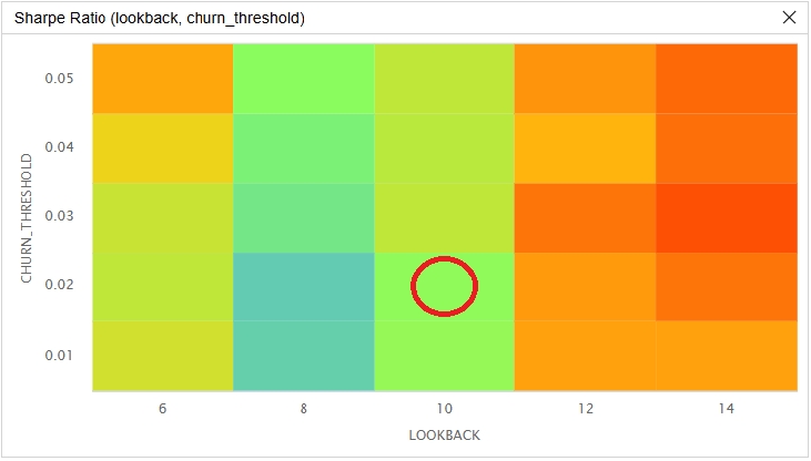
The red circle in the preceding image identifies the parameters we chose as the strategy's default. We chose a 10-day window and a 2% rebalance threshold because both are the values used by Zarattini et al. (2025). That combination produced a 0.729 Sharpe ratio, which is below the grid's 0.746 mean. The grid's maximum of 0.773 sits at a 14-day window and a 3% threshold.
The surface is strikingly flat, with every combination landing between 0.713 and 0.773, so the strategy's risk-adjusted performance barely depends on either parameter. The rebalance threshold is close to inert, moving the average Sharpe ratio by only about one hundredth across its full range. The realized-volatility window has a slightly larger impact, with the strongest cells at the 12-day and 14-day windows and the grid maximum at the 14-day edge, though the pattern is not monotone and the 6-day window scores nearly as well. We do not read a preferred window from this, because the whole spread is small relative to what a decade of returns can resolve, and a maximum sitting at the searched boundary is as consistent with sampling noise as with a real trend.
Every combination in the grid beat the benchmark, and the narrow 0.713 to 0.773 spread means the result does not hinge on the exact window or threshold. The edge over holding the SPY comes from adding a timed short-volatility position to it, and the two signals are what unwind that short during the crises that punish an unconditional short-volatility position. Future research could improve the crude realized-volatility forecast with intraday returns or a GARCH-style model that captures volatility clustering.
References
- Zarattini, C., Mele, A., & Aziz, A. (2025). The Volatility Edge: A Dual Approach for VIX ETNs Trading. Swiss Finance Institute. https://papers.ssrn.com/sol3/papers.cfm?abstract_id=5316487


Jowalz
Thanks for this one — the dual-signal implementation was a great starting point and saved me a lot of time.
My version is here if useful: https://www.quantconnect.com/strategies/682/VIX-Dual-Signal-Premium
Up front: it isn't an improvement on the KPIs. CAGR, Sharpe, Sortino, Alpha, etc., all come out at or below yours — mostly because I added as you have done the SPY overlay, which was carrying a good part of the return. What it is, is somehow more flexible and closer to the paper.
I refactored it and reconciled it line-by-line against Zarattini/Mele/Aziz (SSRN 5316487). Two major things worth flagging:
1. The SPY overlay (`1 + target_weight` when short vol) isn't in the paper or the authors' reference notebook — both hold the remainder in cash and explicitly assume no interest on it. With the overlay on, roughly 76-80% of the book is long SPY on ~90% of days, so a good part of the equity curve is equity beta rather than the volatility premium. Removing it drops CAGR meaningfully but makes the result comparable to Table 3 in the SSRN paper.
2. Short VIXY isn't equivalent to the paper's VIXSHORT. Their proxy is the -1x inverse index (XIV-like, net of 80bp), which resets daily by construction. A static short of a +1x ETN sheds exposure as it profits, so with a 2% rebalance band you systematically under-participate in the drift that generates the return. My realised vol came in at 12% against the paper's 16.4%, which I think is that effect. SVIX (true -1x, from March 2022) or VIX futures directly would be closer.
I also added a few parameters so the paper's variants can be switched between without editing code:
- `sizing_mode` — "dynamic" = Strategy 4 (eVRP + BoC + Sizing); "static" = Strategy 3 (eVRP + BoC) at the fixed 20%/10%
- `sizing_divisor` — the paper's VIX/100 heuristic as a risk dial (VIX/200 conservative, VIX/75 aggressive)
- `long_vol_etn` / `short_vol_etn` with a beta per leg, so short vol can be expressed as short VIXY (1x), long SVXY (2x, since it's -0.5x) or long SVIX (1x) at matched exposure
- `spy_overlay` — on by default to get your original behaviour
- `exposure_band` — the 2% threshold, quoted in vol-exposure terms so it means the same thing whichever leg expresses the trade
One last note for anyone extending the backtest earlier: VIXY only lists from 2011-01-04, so a pre-2011 like in the SSRN paper start silently produces no vol trades at all — and with the SPY overlay on, that turns into a naked long-equity book straight through 2008.
Derek Melchin
The material on this website is provided for informational purposes only and does not constitute an offer to sell, a solicitation to buy, or a recommendation or endorsement for any security or strategy, nor does it constitute an offer to provide investment advisory services by QuantConnect. In addition, the material offers no opinion with respect to the suitability of any security or specific investment. QuantConnect makes no guarantees as to the accuracy or completeness of the views expressed in the website. The views are subject to change, and may have become unreliable for various reasons, including changes in market conditions or economic circumstances. All investments involve risk, including loss of principal. You should consult with an investment professional before making any investment decisions.
To unlock posting to the community forums please complete at least 30% of Boot Camp.
You can continue your Boot Camp training progress from the terminal. We hope to see you in the community soon!