


 Share New Research


Introduction
The literature increasingly attributes the momentum effect of stocks to return extrapolation, the tendency of investors to project past price changes into future expectations. Cannon and Lynch (2025) find that momentum returns are roughly twice as large among stocks that pay no dividends. Inspired by that result, this strategy builds a momentum portfolio from the most liquid US Equities that pay no dividends. Following the Fama-French convention, the strategy calculates its momentum threshold from the NYSE-listed stocks alone and only trades the stocks in its universe with a greater momentum than that threshold. The results show the strategy achieved greater risk-adjusted returns than a buy-and-hold position in the SPY over the last 10 years.
Background
A long line of research since Jegadeesh and Titman (1993) shows that stocks with high returns over the past year continue to outperform over the following month. Behavioral models attribute the effect to return extrapolation. When some investors form beliefs by projecting past returns forward, good news pushes prices up, extrapolators buy into the rise, and the overreaction gradually resolves, producing the drift that momentum strategies harvest.
Cannon and Lynch (2025) add a testable refinement to this story. Extrapolation operates on the price path rather than on total returns, and a dividend stream diverts investor attention away from the price path. They measure extrapolative tendencies with social media sentiment and analyst price targets. Sentiment toward non-dividend-paying stocks, which they call capital-gain stocks, is up to five times more sensitive to past returns than sentiment toward dividend-payers.
If extrapolation drives momentum, the momentum premium should then concentrate in capital-gain stocks. Their portfolio tests confirm it. A momentum strategy earns an average 1.417% per month among capital-gain stocks against 0.684% among dividend-payers, a difference no standard factor model explains.
The strategy in this research post turns that concentration into a long-only monthly rotation. From the 1,000 most liquid US Equities with at least a year of month-end price history, it keeps ordinary common stocks listed on the NYSE, NASDAQ, or AMEX that are priced at $5 or above, excluding financial and utility firms. It classifies a stock as capital-gain if the stock distributed no dividend over the trailing twelve months. Momentum for each stock is
\[ M_{i} = \frac{P_{i,t-2}}{P_{i,t-13}} - 1, \]
where \( P_{i,m} \) is the split- and dividend-adjusted price of stock \( i \) at the end of month \( m \) and \( t \) is the holding month, so the window covers eleven months and skips the most recent one, following the standard convention that avoids short-term reversal. The strategy computes the 95th percentile of momentum using only NYSE-listed stocks, mirroring the NYSE breakpoints common in the academic literature, and buys every capital-gain stock whose momentum exceeds that threshold, equally weighted, rebalancing at each month-end.
Implementation
To implement this strategy, we start by defining a universe of US Equities in the initialize method. We schedule the universe to select constituents on the last trading day of each month and we add a Scheduled Event to rebalance the portfolio at 8 AM Eastern Time (ET) on the same day.
# Add a universe of US Equities.
date_rule = self.date_rules.month_end('SPY')
self.universe_settings.resolution = Resolution.DAILY
self.universe_settings.schedule.on(date_rule)
self._universe = self.add_universe(self._select_assets)
# Add a member to track the momentum of each Equity.
self._momentum_by_symbol = {}
# Add a Scheduled Event to rebalance the portfolio each month.
self.schedule.on(date_rule, self.time_rules.at(8, 0), self._rebalance)
The algorithm maintains an eleven-month momentum indicator for each US Equity. When the universe selection function runs at the end of each month, it updates all the momentum indicators. The update method of the indicator returns a boolean that represents if the indicator has at least twelve month-end prices to provide a momentum score, so the following statement also selects the subset of stocks that have a momentum score ready.
def _select_assets(self, fundamentals: List[Fundamental]) -> List[Symbol]:
    # Update the momentum indicators of all the stocks.
    fundamentals = [
        f for f in fundamentals
        if self._momentum_by_symbol.setdefault(f.symbol, RateOfChange(11)).update(f.end_time, f.adjusted_price)
    ]
The universe then narrows the 1,000 most liquid stocks to just the stocks that:
- are common stocks of US-incorporated, public operating companies,
- have their primary listing on the NYSE, NASDAQ, or AMEX,
- are priced at $5 or above, and
- fall outside the utility and financial sectors, as judged by their SIC codes.
Along the way, the selection records which of the survivors list on the NYSE, because the momentum threshold later comes from that subset alone.
screened_symbols = []
nyse_symbols = set()
for f in sorted(fundamentals, key=lambda f: f.dollar_volume)[-1000:]:
    if (f.has_fundamental_data and
        f.company_reference.country_id == "USA" and
        f.company_reference.company_status == "U" and
        f.security_reference.security_type == "ST00000001" and
        f.security_reference.is_primary_share and
        f.security_reference.exchange_id in {"NYS", "NAS", "ASE"} and
        f.price >= 5 and
        not(4900 <= f.asset_classification.sic <= 4949) and
        not(6000 <= f.asset_classification.sic <= 6999)):
        screened_symbols.append(f.symbol)
        if f.security_reference.exchange_id == "NYS":
            nyse_symbols.add(f.symbol)
Next, we need to classify the stocks into two groups, those that pay dividends and those that don't. A history request pulls the trailing year of dividend distributions for the screened stocks. Any stock that paid at least one dividend in that window counts as dividend-paying, and the rest form the capital-gain group the strategy trades.
dividend_paying_symbols = {
    dividend.symbol
    for dividends_by_symbol in self.history[Dividend](screened_symbols, timedelta(365))
    for dividend in dividends_by_symbol.values()
}
capital_gain_symbols = set(screened_symbols) - dividend_paying_symbols
The universe selection ends by reading each indicator's previous value, computing the 95th percentile of momentum among the NYSE-listed stocks, and returning the capital-gain stocks that exceed it. Reading the indicator's previous value is what lags the window by one month to implement the skip-month convention.
# Get the momentum of t-13 through t-2 for each stock.
momentum_by_symbol = {symbol: self._momentum_by_symbol[symbol].previous.value for symbol in screened_symbols}
# Calculate the 95th percentile of momentum scores using only NYSE-listed stocks.
nyse_momentum_values = [momentum_by_symbol[symbol] for symbol in nyse_symbols]
threshold = np.percentile(nyse_momentum_values, 95)
# Select the stocks that don't pay dividends and have greater momentum than the 95th percentile.
return [symbol for symbol in capital_gain_symbols if momentum_by_symbol[symbol] > threshold]
Finally, the _rebalance method that runs at the end of each month forms an equal-weighted portfolio of the current universe constituents, liquidating the positions that left the selection.
# Each month, form an equal-weighted portfolio of the stocks in the universe.
def _rebalance(self) -> None:
    if self.is_warming_up:
        return
    symbols = self._universe.selected
    weight = 1/len(symbols)
    self.set_holdings([PortfolioTarget(symbol, weight) for symbol in symbols], True)
Results
We backtested the strategy from July 2016 to July 2026. Over that period the strategy earned a 0.602 Sharpe ratio. In contrast, a buy-and-hold position in the SPY over the same time period achieved a 0.552 Sharpe ratio. Therefore, the strategy outperformed the benchmark.
We ran a parameter optimization job to test the sensitivity of the chosen parameters. We tested the momentum lookback \( L \), which forms the momentum window over months \( t-L \) through \( t-2 \), from 6 to 18 in steps of 3, and we tested the NYSE momentum percentile that sets the selection cutoff from 90 to 98 in steps of 2. Of the 25 parameter combinations, 23/25 (92%) produced a greater Sharpe ratio than the benchmark. The following image shows the heatmap of Sharpe ratios for the parameter combinations:
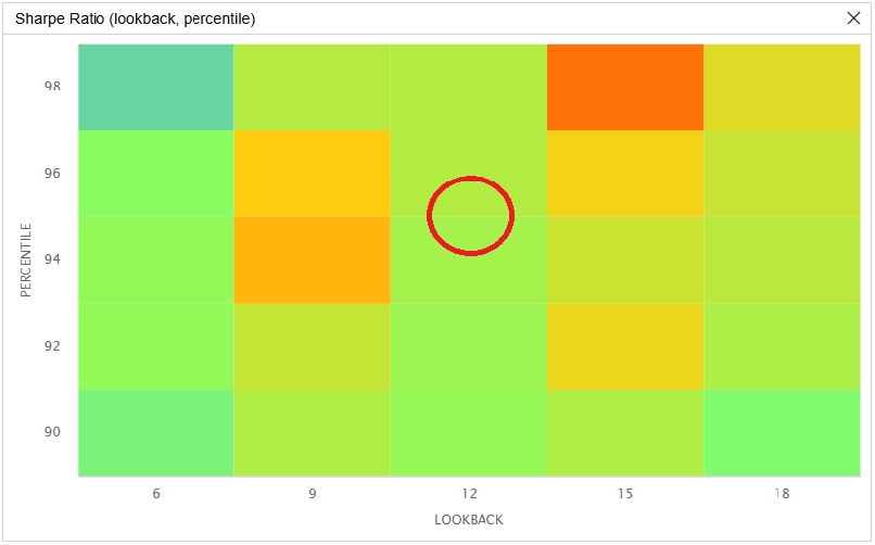
The red circle in the preceding image marks the parameters we chose as the strategy's default. We chose a lookback of 12 months because it matches the \( t-13 \) to \( t-2 \) formation window that is standard in the momentum literature, and a percentile of 95 because it concentrates the portfolio in the strongest capital-gain momentum stocks while retaining enough of them to diversify single-stock risk. The percentile default sits between two tested rows, where the lookback-12 cells produced Sharpe ratios of 0.609 and 0.627, both close to and slightly above the 0.602 the default parameters earned in the full backtest.
The lookback is the more sensitive parameter. Its Sharpe ratio range within a single percentile row reaches 0.325, and the surface is multimodal, with one local peak at a lookback of 15, which produced the best tested cell (0.823 at the 98th percentile), and another at a lookback of 9 (0.754 at the 94th percentile). The percentile matters most near the top of its range. At lookbacks of 15 and 18, the Sharpe ratio generally rises toward the 98th percentile, and the best tested combination sits at the edge of the searched range, so the in-sample optimum may lie beyond it. At a lookback of 6, however, the pattern reverses and the 98th percentile produces the worst cell in the grid (0.498). A plausible explanation for the percentile effect is that a tighter cutoff concentrates the portfolio in the extreme winners, where the extrapolation evidence in Cannon and Lynch (2025) is strongest. Since the same tight cutoff produced both the grid's best cell (lookback 15) and its worst (lookback 6), concentration seems to amplify whatever the ranking contains, rewarding the informative longer windows and punishing the noisy 6-month one.
The strategy outperformed buy-and-hold SPY over the decade tested, and the margin did not depend on a lucky parameter choice, since 92% of the tested combinations also beat the benchmark's Sharpe ratio. The sensitivity analysis still calls for restraint because the best cells cluster at the boundary of the tested grid and the lookback surface is multimodal. Future research could address the strategy's crash exposure, since a concentrated portfolio of extreme winners suffers most when momentum reverses after a market decline. Daniel and Moskowitz (2016) propose managing this risk by scaling the position with volatility. A replacement buffer that keeps an incumbent holding until its momentum falls below a lower percentile would also cut turnover.
References
- Cannon, B., & Lynch, J. (2025). Return Extrapolation and Dividends. Available at SSRN 3816782.
- Daniel, K., & Moskowitz, T. J. (2016). Momentum Crashes. Journal of Financial Economics, 122(2), 221-247.
- Jegadeesh, N., & Titman, S. (1993). Returns to Buying Winners and Selling Losers: Implications for Stock Market Efficiency. The Journal of Finance, 48(1), 65-91.


Derek Melchin
The material on this website is provided for informational purposes only and does not constitute an offer to sell, a solicitation to buy, or a recommendation or endorsement for any security or strategy, nor does it constitute an offer to provide investment advisory services by QuantConnect. In addition, the material offers no opinion with respect to the suitability of any security or specific investment. QuantConnect makes no guarantees as to the accuracy or completeness of the views expressed in the website. The views are subject to change, and may have become unreliable for various reasons, including changes in market conditions or economic circumstances. All investments involve risk, including loss of principal. You should consult with an investment professional before making any investment decisions.
To unlock posting to the community forums please complete at least 30% of Boot Camp.
You can continue your Boot Camp training progress from the terminal. We hope to see you in the community soon!