


 Share New Research


Introduction
Pairing a long position in one market with a short position in another removes most of the risk from the overall market, so the result depends only on which region does better. The strategy in this research post makes that bet on US and international stocks, holding SPY and shorting foreign companies with the lowest return on equity. From October 2009 to October 2026, the dollar-neutral portfolio earned a 3.16% compounding annual return with a beta of 0.01.
Background
The relative performance of US and international stocks depends on differences in economic growth, sector mix, and exchange rates. Exchange rates matter because the US-listed shares of foreign companies move with their home currency. SPY tracks the S&P 500 Index and represents the US side. The international side comes from the large non-US companies whose shares trade in the US but aren't in SPY. Examples include Toyota, SAP and Royal Bank of Canada. Holding equal dollar amounts on each side offsets most of the market's overall direction, so the portfolio's return depends mainly on which side performs better.
Rather than shorting every international stock, the strategy uses profitability to decide which ones to short. Fama and French (2015) and Hou, Xue and Zhang (2015) find that companies with weak profitability earn lower average returns than companies with robust profitability. That makes the least profitable international companies natural candidates for the short side.
We measure profitability with return on equity,
\[ ROE = \frac{NI}{BE}, \]
where \( NI \) is a company's trailing 12-month net income and \( BE \) is the latest book value of its shareholders' equity. A company with negative equity has no meaningful return on equity, so only companies with positive equity are ranked.
Each day, the strategy ranks the non-US companies with a market capitalization above $10 billion by return on equity and shorts every company whose return on equity is below the group's median. The median split lets the short side grow and shrink with the universe instead of holding a fixed number of stocks.
The portfolio holds equal dollar amounts long and short,
\[ w_{SPY} = 0.5 \quad \text{and} \quad w_i = -\frac{0.5}{N}, \]
where \( N \) is the number of non-US companies with below-median return on equity and \( w_i \) is the weight of each of them.
Implementation
To implement this strategy, we start by adding SPY and an ETF constituents universe that tracks its holdings in the initialize method.
# Define some parameters.
self._minimum_market_cap = 10_000_000_000
# Add SPY and add its ETF Constituents universe so we can track the assets in it.
self._spy = self.add_equity('SPY', Resolution.DAILY).symbol
self._etf_constituents = []
self.add_universe(self.universe.etf(self._spy), self._record_etf_constituents)
We then add a fundamental universe that selects the stocks to short each day and a Scheduled Event that rebalances the portfolio at 8 AM Eastern Time (ET) each trading day. We also add a 90-day warm-up so we have SPY's holdings before the first rebalance.
# Add a universe that selects the stocks to short each day.
self.universe_settings.resolution = Resolution.DAILY
self._universe = self.add_universe(self._select_assets)
# Add a Scheduled Event to rebalance the portfolio before the open of each trading day.
self.schedule.on(self.date_rules.every_day(self._spy), self.time_rules.at(8, 0), self._rebalance)
# Add warm-up so we have ETF constituent data before the first rebalance.
self.set_warm_up(timedelta(90))
The _record_etf_constituents universe selection function saves SPY's current holdings and returns an empty list, so the _select_assets method can tell which stocks are in SPY.
def _record_etf_constituents(self, constituents: List[Fundamental]) -> List[Symbol]:
    # Record the ETF constituents so we can use them in the _select_assets selection function.
    self._etf_constituents = [c.symbol for c in constituents]
    return []
Each day, the _select_assets universe selection function selects the stocks that have a market capitalization above $10 billion, positive shareholders' equity, and a trailing 12-month net income. It then returns the non-US companies outside SPY whose return on equity is below the median of that group.
def _select_assets(self, fundamental: List[Fundamental]) -> List[Symbol]:
    if not self._etf_constituents:
        return []
    # Select the stocks above the market cap threshold that have positive equity and a trailing 12-month net income.
    stocks = [f for f in fundamental if f.market_cap > self._minimum_market_cap and not np.isnan(self._return_on_equity(f))]
    # Measure each stock's return on equity.
    return_on_equity = pd.Series({f.symbol: self._return_on_equity(f) for f in stocks})
    # Select the non-US companies outside SPY with below-median profitability for the short side of the portfolio.
    non_us_stocks = [f.symbol for f in stocks if f.symbol not in self._etf_constituents and f.company_reference.country_id != 'USA']
    non_us_profitability = return_on_equity[non_us_stocks]
    return list(non_us_profitability[non_us_profitability < non_us_profitability.median()].index)
The _select_assets method gets each stock's return on equity from the _return_on_equity helper method, which divides the trailing 12-month net income by the latest shareholders' equity. When the equity isn't positive, the method returns no value, so the stock isn't traded.
def _return_on_equity(self, f: Fundamental) -> float:
    # Divide the trailing 12-month net income by the latest shareholders' equity.
    equity = f.financial_statements.balance_sheet.stockholders_equity.value
    return f.financial_statements.income_statement.net_income.twelve_months / equity if equity > 0 else np.nan
The _rebalance method then rebalances the portfolio to hold 50% long SPY and 50% short in equal weights across the current universe constituents. The orders are placed before the open, so they fill at the opening price as market on open orders.
def _rebalance(self) -> None:
    # Hold 50% of the portfolio long SPY and 50% short, split equally across the least profitable foreign stocks.
    targets = [PortfolioTarget(self._spy, 0.5)]
    targets += [PortfolioTarget(symbol, -0.5 / len(self._universe.selected)) for symbol in self._universe.selected]
    # Place trades to rebalance the portfolio.
    self.set_holdings(targets, True)
Results
From October 2009 to October 2026, the strategy earned a 3.16% compounding annual return with a beta of 0.01. Therefore, it achieved a positive return with effectively no exposure to the overall market.
We ran a parameter optimization job to test the sensitivity of the chosen parameters. We tested minimum market caps from $5 billion to $15 billion in steps of $1 billion. All 11 values earned a positive return, between 2.63% and 3.66% a year, with betas of 0.02 or less. The following image shows the compounding annual return for each value:
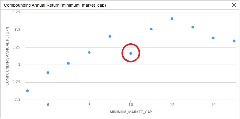
The red circle in the preceding image identifies the parameter we chose as the strategy’s default. We chose a minimum market cap of $10 billion because it’s where large-cap stocks start in FINRA’s categories. SPY holds large US companies, so the floor limits the short side to large international companies too.
The return rises as the floor increases from $5 billion to $12 billion and then eases slightly up to $15 billion. A floor of $12 billion earned the most at 3.66% a year, while the $10 billion floor we use earned 3.16% and sits below both of its neighbors. That dip suggests the differences of a few tenths of a percent between nearby floors are partly noise. A plausible explanation for the upward slope is that a lower floor admits smaller international companies. Their returns may depend more on their own businesses than on the split between US and international stocks that drives the strategy.
The strategy earned a positive return with almost no market exposure at every floor we tested, so its result doesn't depend on one particular floor. Future research could separate the effect of exchange rates from the stocks' own returns. It could also give the two sides the same sector weights, so differences in sector mix don't drive the result. Finally, splitting the short side by region would show which countries contribute most to the return.
References
- Fama, E. F., & French, K. R. (2015). A five-factor asset pricing model. Journal of Financial Economics, 116(1), 1-22. https://doi.org/10.1016/j.jfineco.2014.10.010
- Hou, K., Xue, C., & Zhang, L. (2015). Digesting anomalies: An investment approach. The Review of Financial Studies, 28(3), 650-705. https://doi.org/10.1093/rfs/hhu068


Team Quantpedia
The material on this website is provided for informational purposes only and does not constitute an offer to sell, a solicitation to buy, or a recommendation or endorsement for any security or strategy, nor does it constitute an offer to provide investment advisory services by QuantConnect. In addition, the material offers no opinion with respect to the suitability of any security or specific investment. QuantConnect makes no guarantees as to the accuracy or completeness of the views expressed in the website. The views are subject to change, and may have become unreliable for various reasons, including changes in market conditions or economic circumstances. All investments involve risk, including loss of principal. You should consult with an investment professional before making any investment decisions.
This discussion is closed