Introduction
The iShares Top 20 U.S. Stocks ETF (TOPT) launched on October 23, 2024. It is composed of the 20 largest U.S. companies by market capitalization within the S&P 500 Index. It is effectively long the market capitalization factor within the SPY universe. In this research post, we simulate the historical performance of TOPT and attempt to outperform it by optimizing the portfolio’s exposures to multiple factors within the same universe of assets.
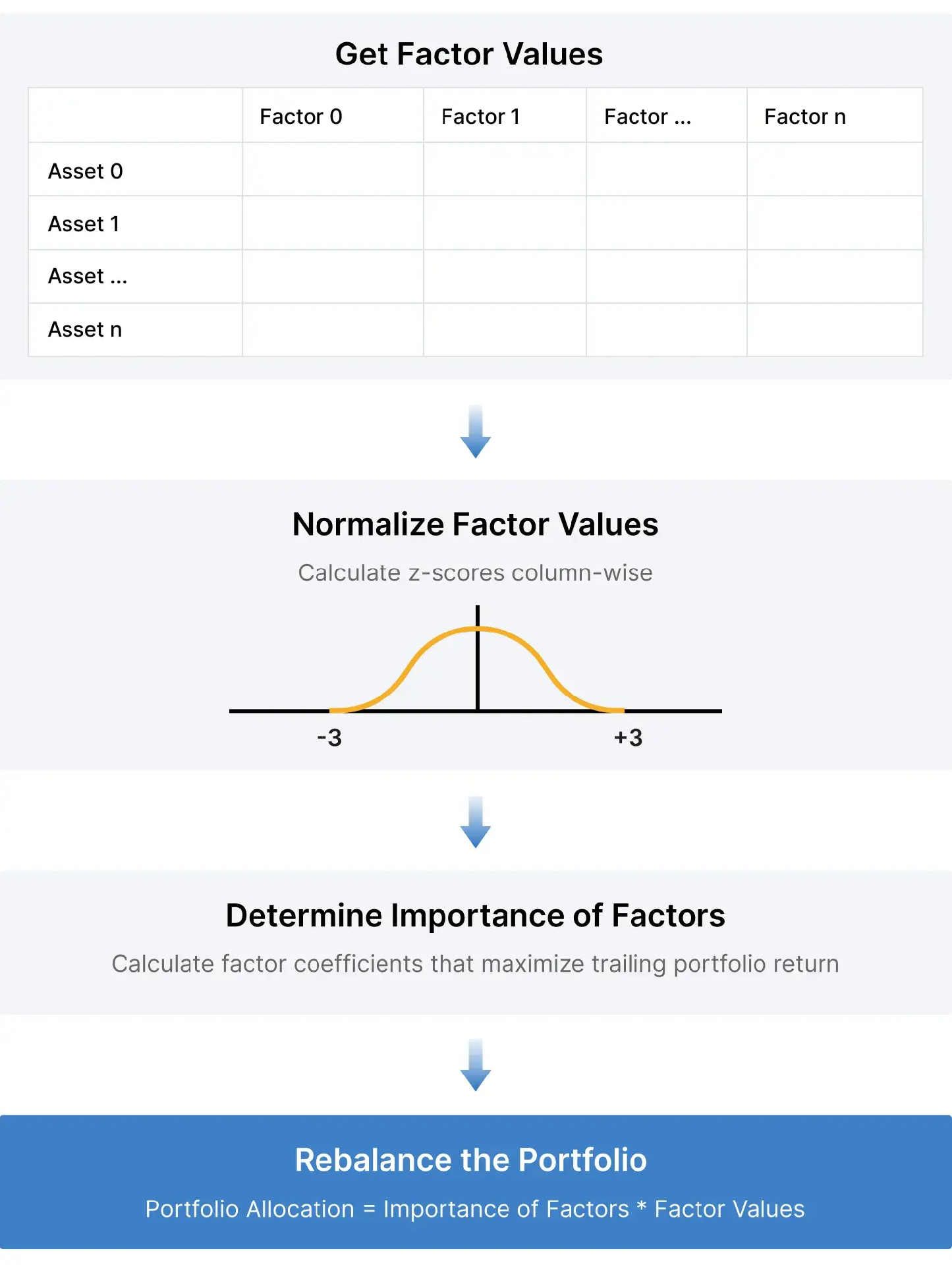
The project discussed in this post is a factor experimentation framework. The optimizer determines the exposure to give to each factor in order to maximize the trailing returns of the portfolio. The algorithm then uses these factor exposure coefficients and the current factor values of each asset to determine the target portfolio weight of each asset during a monthly rebalance.
Implementation

To implement this strategy, we start by adding an ETF constituents universe in the initialize method. We select the largest US Equities in the SPY ETF.
self.universe_settings.resolution = Resolution.HOUR
universe_size = self.get_parameter('universe_size', 20)
self._universe = self.add_universe(self.universe.etf(spy, universe_filter_func=lambda constituents: [c.symbol for c in sorted([c for c in constituents if c.weight], key=lambda c: c.weight)[-universe_size:]]))
To end the initialize method, we create a Scheduled Event to rebalance the portfolio at the start of each month. We’re using hourly data.
self.schedule.on(self.date_rules.month_start(spy), self.time_rules.after_market_open(spy, 31), self._rebalance)In the on_securities_changed method, we create some factors for each asset that enters the universe.
def on_securities_changed(self, changes):
    for security in changes.added_securities:
        security.factors = [MarketCapFactor(security), SortinoFactor(self, security.symbol, self._lookback)]
These factors are defined in the project’s factors.py file. For example, the MarketCapFactor simply returns the market cap value from Morningstar.
class MarketCapFactor:
    def __init__(self, security):
        self._security = security

    @property
    def value(self):
        return self._security.fundamentals.market_cap
There are few steps in the _rebalance method that runs at the start of each month. First, it gets the factors values of each asset in the universe.
factors_df = pd.DataFrame()
for symbol in self._universe.selected:
    for i, factors in enumerate(self.securities[symbol].factors):
        factors_df.loc[symbol, i] = factors.value
Second, it standardizes the factor values to generate z-scores, which describe a value's relationship to the mean of a group of values, measured in terms of standard deviations from the mean. After this operation, assets with the above-average values for a factor have positive z-scores for the factor. The optimizer and portfolio construction logic takes the dot product of these z-scores and the portfolio weights, which means assets with greater z-scores for all factors end up with the greatest weight in the portfolio.
factor_zscores = (factors_df - factors_df.mean()) / factors_df.std()Third, it runs an optimization to find the factor coefficients that maximize the trailing return of the portfolio.
trailing_return = self.history(list(self._universe.selected), self._lookback, Resolution.DAILY).close.unstack(0).pct_change(self._lookback-1).iloc[-1]
num_factors = factors_df.shape[1]
factor_weights = optimize.minimize(lambda weights: -(np.dot(factor_zscores, weights) * trailing_return).sum(), x0=np.array([1.0/num_factors] * num_factors), method='Nelder-Mead', bounds=Bounds([0] * num_factors, [1] * num_factors), options={'maxiter': 10}).x
Lastly, it calculates the portfolio weights and places trades to rebalance the portfolio. The portfolio is designed to be long-only with 100% exposure.
portfolio_weights = (factor_zscores * factor_weights).sum(axis=1)
portfolio_weights = portfolio_weights[portfolio_weights > 0]
self.set_holdings([PortfolioTarget(symbol, weight/portfolio_weights.sum()) for symbol, weight in portfolio_weights.items()], True)
Results
We backtested the algorithm from January 2015 to the current day. The benchmarks we chose were:
- Buy and hold the SPY (0.547 Sharpe ratio)
- An equal-weighted portfolio of the 20 largest constituents of the SPY (0.616 Sharpe ratio)
- A market cap-weighted portfolio of the 20 largest constituents of the SPY (0.675 Sharpe ratio)
In contrast, our factor optimization algorithm achieved a 0.764 Sharpe ratio, outperforming the three preceding benchmarks. To test the sensitivity of the parameters chosen, we ran a two parameter optimization jobs on the lookback period and universe size.
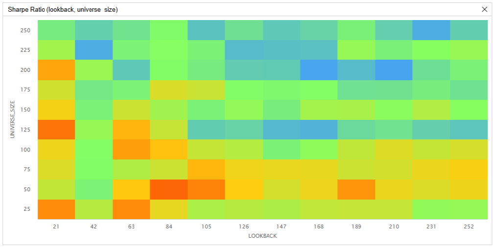
In the first parameter optimization, we tested lookback periods from 21 trading days (1 month) to 252 trading days (1 year) in steps of 21 trading days and we tested the universe size from 25 (5% of the SPY) to 250 (50% of the SPY) in steps of 25. Of the 120 parameter combinations, 74 (61.7%) outperformed the buy and hold benchmark, 51 (42.5%) outperformed the equal-weighted benchmark, and 28 (23.3%) outperformed the market cap-weighted benchmark.
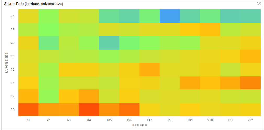
To optimize around the range of the TOPT universe constituents, the second parameter optimization tested the same lookback periods and tested the universe size from 10 to 24 in steps of 2. Of the 96 parameter combinations, 89 (92.7%) outperformed the buy and hold benchmark, 83 (86.5%) outperformed the equal-weighted benchmark, and 72 (75%) outperformed the market cap-weighted benchmark.
The following images shows the heatmaps of Sharpe ratios for the parameter combinations:


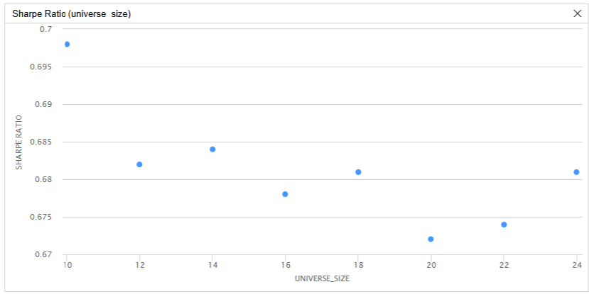
These parameter optimization results show the Sharpe ratio can be sensitive to changes in the parameter values and the strategy tends to achieve the greatest Sharpe ratio with a small universe and lookback period. However, there is no obvious center of mass. Even if we run a parameter optimization job on benchmark #3 (the market cap-weighted portfolio of the 20 largest constituents of the SPY), we have similar findings. In fact, a universe size of 20 for this benchmark has the lowest Sharpe ratio out of all the universe sizes tested.

As a result, investors may outperform TOPT by using an even smaller universe size than 20.
Further Research
The algorithm currently uses the market cap and Sortino ratio as the factors for each asset. To test other factors, define a new factor class in the factors.py file and then construct the new factor in the on_securities_changed method. The optimization logic is designed so that factor values are correlated with asset returns (larger values = greater expected returns), so engineer new factors in this way.


.ekz.
Thanks for this Derek Melchin. A very inspiring share. Using the Nelder-Mead approach for maximizing factor coefficients was a revalation – I definitely learned something here.
Here's a version that should also inspire others – it uses a KER factor and FCFYield factor instead, and based on only the top 5 weighted SPY constituents.
Decebal Mihailescu
is it possible to optimize for shorting the weakest constituents?
I'm not sure how to apply it to optimize.minimize(….
Derek Melchin
The material on this website is provided for informational purposes only and does not constitute an offer to sell, a solicitation to buy, or a recommendation or endorsement for any security or strategy, nor does it constitute an offer to provide investment advisory services by QuantConnect. In addition, the material offers no opinion with respect to the suitability of any security or specific investment. QuantConnect makes no guarantees as to the accuracy or completeness of the views expressed in the website. The views are subject to change, and may have become unreliable for various reasons, including changes in market conditions or economic circumstances. All investments involve risk, including loss of principal. You should consult with an investment professional before making any investment decisions.
To unlock posting to the community forums please complete at least 30% of Boot Camp.
You can continue your Boot Camp training progress from the terminal. We hope to see you in the community soon!