


Research conducted by Ethan Huang, Mentored by Rudy Osuna - Triton Quantitative Trading @ UC San Diego
Introduction
The Log-Periodic Power Law Singularity (LPPLS) has been shown to be predictive of financial bubbles and systemic market crashes throughout history, including research done in the 2008 Great Recession. The LPPLS model assumes that market bubbles are characterized by a transition from steady linear growth to super-exponential acceleration, driven by positive feedback loops. In an age of social media, this phenomenon becomes more likely due to the hype created by economic swings. In these regimes, volatility oscillates with increasing frequency as the system approaches a critical singularity, the proposed bubble pop. We can extrapolate this idea into modern markets which have gone through periodic trends of volatility through American economic uncertainty and AI hype post-2023.
Method
The standard LPPLS equation is defined as:
\[\ln(p(t)) = A + B(t_c - t)^m + C(t_c - t)^m \cos(\omega \ln(t_c - t) - \phi)\]
The LPPLS model is dependent on 7 different parameters:
- \(A\) is the predicted maximum price at the crash date.
- \(B\) is the magnitude of the power law trend.
- \(t_c\) is the predicted crash date, which is what we want to predict.
- \(\omega\) is the periodicity of the price oscillations before the crash.
- \(C\) is the volatility of the oscillations.
- \(m\) is the degree of the super-exponential growth.
- \(\phi\) is the phase shift.
Instead of optimizing each parameter individually, we induce a hybrid optimization approach by using Ordinary Least Squares to solve for the linear parameters. By applying the trigonometric identity \(\cos(a-b) = \cos(a)\cos(b) + \sin(a)\sin(b)\), we rewrite the LPPLS equation to:
\[y(t) = A + B(t_c - t)^m + C_1(t_c - t)^m \cos(\omega \ln(t_c - t)) + C_2(t_c - t)^m \sin(\omega \ln(t_c - t))\]
This provides 4 linear terms we can optimize using a matrix algebra approach \((A, B, C_1, C_2)\), leaving only 3 non-linear terms to be determined via a 3D optimizer.
We can pack this information into three distinct matrices. The vector \(y\) is a \(100 \times 1\) matrix of historical log-prices, while \(X\) is a \(100 \times 4\) matrix representing the coefficients of the LPPLS trend, where the first column encodes the bias term (all ones), the second captures the power-law trend, the third holds the cosine term, and the fourth holds the sine term. Finally, \(Z\) is a \(4 \times 1\) matrix of the unknowns \((A, B, C_1, C_2)\).
Together, these form the relationship \(y = XZ\). Using the normal equation, we solve for \(Z\) and introduce a weight matrix \(W\), a diagonal matrix designed to upweight more recent trading days:
\[Z = (X^T W X)^{-1} (X^T W y)\]
We perform this calculation for each \(X\) matrix passed into the function. This \(X\) matrix is constructed from the non-linear parameters \((t_c, m, \omega)\) via parameter estimation.
Since the LPPLS function is often non-convex, we are met with a computational challenge. For each of the non-linear parameters, we initialize starting seeds over a plausible range, ensuring that our model follows the implied physics of the LPPLS model. This includes keeping \(m < 1\) for our super-exponential assumption. For each of our guesses, we compile them into the \(X\) matrix and use it to calculate the linear parameters. The best model is selected via minimization of the Ordinary Least Squares between the LPPLS model and the true prices of the last 100 trading days.
The LPPLS signal is recognized as actionable if three conditions are met:
1. The crash date (\(t_c\)) is predicted within 30 days.
2. The goodness-of-fit metric (\(R^2\)) is sufficiently high.
3. The physics constraints (\(m\) and \(\omega\)) are within reason for a bubble interpretation.
When these conditions are met, we liquidate our long portfolio of the specific Equity and enter a small short position. Otherwise, we fall back to the regime-filter logic of a 50-day EMA and 200-day EMA. If we have a short position but the macro trend is up, we cover the short and re-enter a long position.
The portfolio is rebalanced weekly over a universe of the 100 most liquid Equities priced over $10 over the last week. This gives us exposure to a wide variety of sectors and the most relevant ones in the market.
Results
The simplest baseline for a financial algorithm is a buy-and-hold position over the SPY on the same 5-year interval [backtest link]. SPY achieved a Sharpe Ratio of \(0.4\) with a maximum drawdown of \(24.5\%\). The LPPLS strategy's Sharpe of \(0.503\) modestly outperforms this benchmark, though at the cost of significantly higher drawdown (\(51.7\%\)) during the bearish 2022 market, showing the algorithm's high volatility in both market types.
We further compare against the regime filter alone, a 50-day / 200-day EMA crossover applied to the same universe of the 100 most liquid Equities [backtest link]. This crossover strategy achieved a Sharpe Ratio of \(0.16\) with a maximum drawdown of \(29.1\%\). This comparison clarifies how much of the strategy's performance is actually attributed to LPPLS bubble detection versus the EMA buying logic.
As a third reference, we evaluate an equal-weighted buy-and-hold allocation across the same 100-Equity universe [backtest link]. This benchmark achieved a Sharpe Ratio of \(0.015\) with a maximum drawdown of \(38.7\%\). Comparing this baseline measures whether or not the LPPLS performance is simply due to holding a valuable, diversified set of assets.
We ran a parameter optimization job to test the sensitivity of the chosen parameters. We tested a window size of 70 to 140 in steps of 10, and an R2 threshold between 0.65 and 0.9 in steps of 0.05, making it 7 steps in each dimension. Of the 48 parameter combinations, 29/48 (60.4%) produced a greater Sharpe Ratio than the benchmark. The following image shows the heatmap of Sharpe Ratios for the parameter combinations:
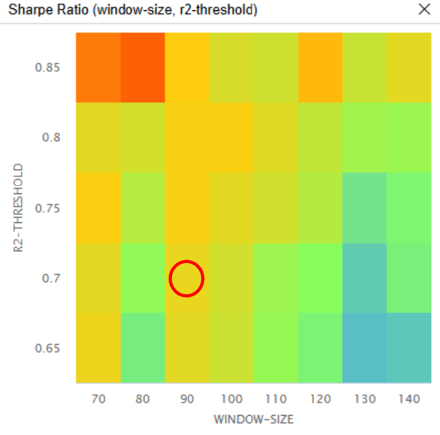
The red circle in the preceding image identifies the parameters we chose as the strategy's default. We chose a window size of 100 and an R2 threshold of 0.7 because it was in the center of an area of the least sensitive parameter combinations.
Given the large amount of hyperparameters in the strategy, this HPO tells us that this model might struggle to adapt in certain financial markets. Although LPPLS shows certain predictive qualities, there is an architectural discrepancy in the way we process the information.
Conclusion
In conclusion, the LPPLS technique we tested for has the potential to outperform a buy-and-hold SPY approach.
However, the strategy's risk metrics highlight the difficulty in attempting to turn profit in bubble prediction. While the LPPLS equation is theoretically robust from the mathematical standpoint, its practical execution in this backtest resulted in a \(51.7\%\) maximum drawdown and a Probabilistic Sharpe Ratio of \(12.5\%\). This variance indicates that while the model quantitatively calculates the presence of a bubble, shorting the market based on the critical time \(t_c\) remains highly susceptible to noise. Being imprecise too early or too late in a bubble prediction causes the model to lose out on profits either from missing out on continued growth or absorbing pains of bubble drawdown.
Ultimately, this research proves that the LPPLS framework possesses some predictive validity as a structural indicator of market trends. To transition this strategy from a theoretical framework to a viable live-traded algorithm, future iterations must focus on variance reduction. Integrating dynamic position sizing and different exit conditions will be essential to allow this algorithm to give a realistic edge over the market.
References
Sornette, D., Cauwels, P., & Smiber, G. (2024). Log-periodic power law singularity (LPPLS) model for financial bubbles. SSRN. https://papers.ssrn.com/sol3/papers.cfm?abstract_id=4734944


Stahl
Hello Rudy, nice work! Thanks for sharing.
Have you looked into this paper [2510.10878] Identifying and Quantifying Financial Bubbles with the Hyped Log-Periodic Power Law Model
It is based on the same Sornette's LPPL model, adding a “Hype” index based on NLP sentiment value. I had no time to implement it on QC yet. if you do, I would be interested ;-)
Marco Cigolini
Hello Rudy, thanks for sharing! The sharpe ratio could be improved by applying a progressive incremental exposition to reduce the DD; also you could try to refine the strategy by backtesting with the support of cluster filters that can trigger the exposition increment. Just a thought. Regards, Marco
Triton Quantitative Trading
The material on this website is provided for informational purposes only and does not constitute an offer to sell, a solicitation to buy, or a recommendation or endorsement for any security or strategy, nor does it constitute an offer to provide investment advisory services by QuantConnect. In addition, the material offers no opinion with respect to the suitability of any security or specific investment. QuantConnect makes no guarantees as to the accuracy or completeness of the views expressed in the website. The views are subject to change, and may have become unreliable for various reasons, including changes in market conditions or economic circumstances. All investments involve risk, including loss of principal. You should consult with an investment professional before making any investment decisions.
To unlock posting to the community forums please complete at least 30% of Boot Camp.
You can continue your Boot Camp training progress from the terminal. We hope to see you in the community soon!