Volatility-Targeted QQQ–TLT Rotation with a Multi-Scale CNN-LSTM Forecast

Research conducted by: Sourish Suri, Antara Chhabra, Jaden Chung, Tanuj Gaudani - Mentored by Rudy Osuna - Triton Quantitative Trading @ UC San Diego

Introduction

This research presents a volatility-targeting trading strategy that combines a deep learning CNN-LSTM model with monthly walk-forward optimization to dynamically allocate between QQQ (Nasdaq-100 ETF) and TLT (long-duration Treasury ETF). The model learns multi-scale temporal patterns in daily Parkinson Volatility. Parkinsons Volatility is a range-based estimator that measures intraday price dispersion from the daily high-low range rather than close-to-close returns. to forecast short-term market turbulence, scaling equity exposure inversely to predicted volatility. This work draws on techniques from HARNet (Reisenhofer et al., 2022), which demonstrated the viability of convolutional neural networks for realized volatility forecasting.

Background

The core hypothesis is that equity exposure should scale inversely with predicted market volatility. By framing allocation decisions as a volatility forecasting task rather than a directional prediction task, we avoid many of the pitfalls of classical price-prediction models while leveraging the well-documented phenomenon of volatility clustering in financial time series.

To model this behavior, we employ a CNN-LSTM hybrid architecture. A Convolutional Neural Network (CNN) is designed to detect local temporal patterns. When applied to time series data, convolutional filters scan across sequences to identify recurring short-term structures such as volatility bursts and sudden range expansions. Different kernel sizes allow the network to capture patterns at multiple temporal scales simultaneously.

A Long Short-Term Memory (LSTM) network is specifically designed to model sequential dependencies. Unlike standard neural networks, LSTMs maintain a memory state that evolves over time, allowing them to capture persistence and temporal dynamics. This is a critical feature when modeling financial volatility, which exhibits clustering and regime dependence.

By combining CNN layers with an LSTM layer, the model first extracts multi-scale local volatility features and then learns how these features evolve over time. This hybrid design is particularly well-suited for volatility forecasting, where both short-term shocks and longer-term persistence play important roles.

Implementation

The strategy follows a sequential pipeline that passes 22-bar rolling windows of daily Parkinson volatility through parallel convolutional layers before feeding the extracted features into a recurrent LSTM layer. Three convolutional filters operate in parallel:

1. A short filter (kernel size 3) captures day-to-day volatility bursts and rapid regime shifts
2. A medium filter (kernel size 5) captures weekly volatility dynamics
3. A long filter (kernel size 22) captures broader monthly regime behavior

After the convolutional block extracts multi-scale features, they are concatenated and fed into an LSTM layer. The LSTM acts as memory, modeling the persistence and temporal evolution of volatility. Fully connected layers then compress the LSTM hidden state into a single scalar representing the forward volatility forecast. Position sizing is a continuous function of this forecast.

1. Capital Initialization and Data Handling

The algorithm subscribes to daily-resolution QQQ and TLT data. QQQ serves as the risky equity leg; TLT serves as the volatility hedge. A rolling session of 1,300 daily bars is maintained to support model training and the Parkinson's custom indicator. The algorithm is warmed up with four years of historical data before live trading begins.

self._qqq = self.add_equity("QQQ", Resolution.DAILY)
self._hedge = self.add_equity("TLT", Resolution.DAILY)
self._qqq.session.size = 1300

The Parkinson indicator is registered directly against the QQQ security so that it updates automatically on every bar. Each daily observation is summarized by a single scalar volatility estimate rather than a four-dimensional OHLC vector: 

\[X_t = \text{PV}_t\]

where \(\text{PV}_t\) denotes the Parkinson volatility estimate at bar \(t\).

2. Parkinson Volatility Estimator

Rather than constructing the volatility signal from squared intraday returns, the strategy uses the Parkinson high-low range estimator, which is more statistically efficient because it exploits the full intraday price range. For each daily bar it is defined as: \[\text{PV}_t = \sqrt{\frac{1}{4\ln 2}\left(\ln\frac{H_t}{L_t}\right)^2}\] where \(H_t\) and \(L_t\) are the daily high and low prices. A small epsilon guard prevents numerical instability when the intraday range approaches zero. The estimator is computed once per bar and stored in a rolling window, from which both the training dataset and live prediction windows are drawn.

3. Target Construction

The model predicts the mean Parkinson volatility over the next 22 bars. The target is log-transformed to compress the right tail of the volatility distribution and stabilize training: 

\[y_i = \ln\!\left(\frac{1}{H}\sum_{j=0}^{H-1}\text{PV}_{i+j}\right)\] 

where \(H=22\) is the future horizon. This corresponds directly to:

y_data.append(np.log(np.mean(park_arr[i:i + self.future_horizon])))

At inference time the log prediction is exponentiated to recover the raw volatility estimate.

4. Input Normalization

Normalization is applied independently to each rolling window of 22 bars to prevent scale dominance from high-volatility regimes and to improve training stability. A small constant \(\epsilon = 10^{-6}\) is added to the denominator to prevent numerical instability when standard deviation approaches zero: 

\[\tilde{X}_i = \frac{X_i - \mu_i}{\sigma_i + 10^{-6}}\]

This ensures the model learns structural volatility patterns rather than absolute volatility levels. The same normalization is applied at inference time.

5. Model Architecture

The model receives a 22-bar rolling window of daily Parkinson volatility values (shape: \(22 \times 1\)). Three parallel convolutional layers extract multi-scale temporal features using kernel sizes 3, 5, and 22. The long kernel directly matches the monthly lookback, giving the network an explicit long-horizon view of the volatility process. The outputs are concatenated before being passed to the LSTM layer:

\[F = \textrm{Concat}(\textrm{Conv}_3(X),\ \textrm{Conv}_5(X),\ \textrm{Conv}_{22}(X))\]

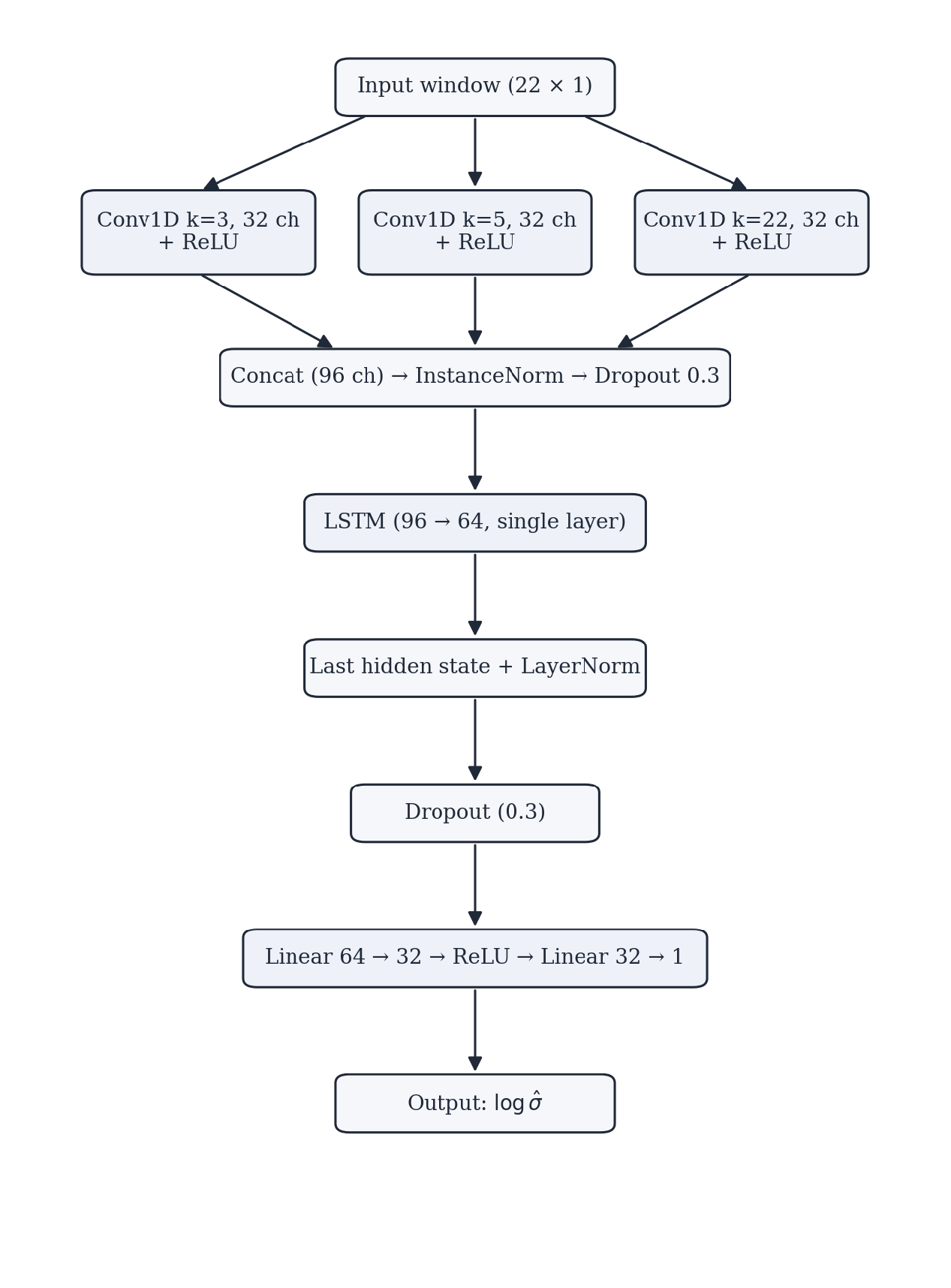
Each convolutional layer produces 32 feature channels, yielding 96 total after concatenation. The concatenated features are instance-normalized and dropout-regularized (rate 0.3) before being passed to a single-layer LSTM with hidden size 64. The LSTM captures temporal dependencies and volatility persistence, modeling the sequential nature of financial time series. Only the final hidden state is retained, layer-normalized, passed through a second dropout (rate 0.3), and mapped to a scalar log-volatility prediction through a small fully connected head:

self.fc = nn.Sequential(
    nn.Linear(64, 32),
    nn.ReLU(),
    nn.Linear(32, 1)
)

6. Training Procedure

The model is retrained monthly, scheduled 30 minutes before market open on the first trading day of each month. The dataset is split chronologically into a 70% training set and a 30% validation set, with the most recent windows held out for validation to prevent data leakage. Within each epoch the training set is reshuffled and processed in mini-batches of size 256. Early stopping with a patience of 6 epochs is applied to reduce overfitting, and training is capped at 50 epochs. Gradient norms are clipped to a unit norm to prevent gradient explosion. The loss function is the mean squared error between predicted and actual log-volatility:

\[\mathcal{L} = \frac{1}{N} \sum_{i=1}^{N} \left(\hat{y}_i - y_i\right)^2\]

Implemented as:

loss_fn   = nn.MSELoss()
optimizer = torch.optim.Adam(self.net.parameters(), lr=1e-3)

The best checkpoint (lowest validation MSE) is restored at the end of training. Train loss, validation loss, and Spearman rank correlation on the validation set are plotted as diagnostics after each training cycle.

7. Walk-Forward Optimization

Because the optimal target volatility shifts across market regimes, it is recalibrated monthly via a grid search over the 65 most recently completed daily bars. The candidate target volatility levels evaluated are 0.08, 0.10, 0.12, 0.14, and 0.16. For each candidate level \(\sigma^*\), position sizes are simulated using the 22-bar rolling mean of the Parkinson estimator (not the model output) as the vol forecast, annualized by \(\sqrt{252}\):

\[\bar{\sigma}_t = \sqrt{252}\cdot\frac{1}{L}\sum_{j=0}^{L-1}\text{PV}_{t-j}, \qquad w_t = \text{clip}\!\left(\frac{\sigma^*}{\bar{\sigma}_t},\ 0,\ 1\right)\]

with \(L=22\). Strategy returns are computed as \(w_t \cdot r_{t+1}\), where the position sized at the close of bar \(t\) earns the return from bar \(t\) to bar \(t+1\). Each candidate is evaluated by its Calmar ratio (annualized return divided by maximum drawdown):

\[\text{Calmar}_i = \frac{\bar{r}_i \cdot 252}{\left|\min_t\!\left(\dfrac{\text{Equity}_t}{\max_{s \leq t}\text{Equity}_s} - 1\right)\right|}\]

The candidate with the highest Calmar ratio is selected as the raw target vol. To dampen month-to-month noise in the WFO output, the raw target is passed through a 3-month simple moving average; the smoothed value \(\sigma_{\text{target}}\) is used here to size our positions:

self._target_vol_sma.update(bars[-1].end_time, raw_vol)
self._target_vol = self._target_vol_sma.current.value

8. Trading Logic

On every daily bar, the algorithm fetches the 22 most recent Parkinson values, normalizes them, and passes them through the trained HARNet. The raw log-volatility prediction is exponentiated to recover the daily volatility estimate. The raw forward volatility forecast at time \(t\) is:

\[\hat{\sigma}_t = \exp\!\left(f_{\theta}(X_t)\right)\]

where \(f_{\theta}\) represents the trained CNN-LSTM model parameterized by weights \(\theta\). This prediction is then smoothed over a 5-bar simple moving average to reduce signal noise, yielding \(\tilde{\sigma}_t\). The smoothed estimate is annualized and used to compute the target QQQ allocation weight:

\[w_t = \text{clip}\!\left(\frac{\sigma_{\text{target}}}{\max\!\left(\tilde{\sigma}_t \cdot \sqrt{252},\ \epsilon\right)},\ 0,\ 1\right)\]

where \(\sigma_{\text{target}}\) is the (3-month smoothed) WFO-selected target volatility, \(\tilde{\sigma}_t\) is the 5-bar smoothed model prediction, and \(\epsilon = 10^{-6}\) is a small constant that prevents division by zero. This mechanism reduces QQQ exposure during volatile regimes and increases it during stable conditions. The remainder is allocated to TLT, so the portfolio is fully invested at all times:

targets = [PortfolioTarget(self._qqq, target_weight), PortfolioTarget(self._hedge, 1 - target_weight)] 
self.set_holdings(targets)

Results

To test the long term performance of our strategy, we ran a 19+ year backtest (from 2007-present day). The earliest backtest we can do is January 1st, 2007 as the data feed for TLT starts in late 2002 and we need a 4 year warmup period to warmup the Market Session. In a 19 year backtest, our CNN-LSTM model (0.644) achieves a higher sharpe ratio than Buy-and-Hold QQQ (0.591). In net profit our CNN-LSTM model underperforms, which is to be expected as we are only adding a Treasury Bond to reduce risk.

To put our algorithm to the test we can take it a step forward and narrow down on the performance specifically in crisis periods. We will be testing our strategy against the benchmark across 14 different crisis events highlighted in the QuantConnect Backtesting Report.

Crisis periods (by Sharpe Ratio):

We only manage to mitigate ~40% of the periods above with our volatility forecasting model over the benchmark in the last 19+ years. The periods above are all the high volatility periods, if we isolate away only crisis events of high drawdown (Global Financial Crisis 2007, Flash Crash 2010, Fukushima Meltdown 2011, U.S. Credit Downgrade 2011, ECB IR Event 2012, European Debt Crisis 2014, Market Sell-Off 2015, COVID-19 2020, Russia Invades Ukraine 2022-2023) the model outperforms in 5 of 9 drawdown windows. In trending bull markets, such as New Normal 2014-2019, Post-COVID Run-up 2020-2021, AI Boom 2022-Present, etc., the model underperforms the QQQ benchmark which is expected as any small allocation to TLT will drag the performance. 

Conclusion

This research demonstrates that with only adding one financial instrument, 20+ Year Treasury Bond TLT, our CNN-LSTM architecture trained on Parkinson volatility targets has potential to be used as a volatility forecasting filter, increasing our sharpe ratio over the passive QQQ buy-and-hold benchmark. The algorithm achieved a Sharpe Ratio of 0.644 over a 19-year window encompassing numerous different market conditions and crisis periods. For this paper, this algorithm was kept fairly simple with minimal assets. Future work would investigate extending the framework to a universe of top dollar volume Equities rather than a single ETF and exploring other hedging instruments to broaden the strategy's diversification and risk-adjusted potential.

References

Pik, J., Chan, E. P., Broad, J., Sun, P., & Singh, V. (2025). Hands-on AI trading with Python, QuantConnect and AWS. John Wiley & Sons Inc.

Guo, Q., Lei, S., Ye, Q., & Fang, Z. (2021). MRC-LSTM: A hybrid approach of multi-scale residual CNN and LSTM to predict Bitcoin price. arXiv:2105.00707.