


 Share New Research


Introduction
Momentum is one of the most durable market anomalies, yet its long-short form has weakened as asset correlations have risen. This strategy refines a cross-asset ETF momentum approach across a fixed set of 13 Equity, bond, commodity, and currency ETFs. Each month, it ranks the ETFs by an average of their 3, 6, 9, and 12-month total returns, holds the top four equal-weighted, and selectively shorts the single worst ETF at a reduced 30% weight when an intra-market correlation filter signals a momentum-favorable regime. This design follows Pauchlyová and Vojtko (2025). The results show that from July 2007 to June 2026, the strategy produced a 0.498 Sharpe ratio, outperforming a buy-and-hold position in the SPY benchmark.
Background
Momentum rests on a simple empirical regularity, that assets which have outperformed recently tend to keep outperforming over the following weeks and months, while recent laggards tend to keep lagging. The natural way to harvest this is a long-short portfolio that buys the winners and shorts the losers. In practice, the long-short version of ETF momentum disappoints. The long leg is robust on its own, but the short leg tends to drag on returns, because shorting recent losers is profitable only in specific market conditions and is otherwise a costly bet against assets that quietly recover.
The refinement keeps the long leg as the core engine and treats shorting as a conditional hedge rather than a permanent position. It averages momentum across several lookback periods, which keeps the ranking from hinging on a single noisy window, and it adds an intra-market correlation filter that decides when the short leg is worth carrying. Those two components convert a weak long-short strategy into a long-biased one that adds a short hedge only when the cross-section of ETFs is behaving in a way that historically rewards momentum.
Cross-Asset Momentum Ranking
Each month, the algorithm scores every ETF by the average of its trailing 3, 6, 9, and 12-month total returns. Writing \( P_{i,t} \) for the split and dividend-adjusted price of ETF \( i \), the score is
\[ M_i = \frac{1}{4} \sum_{k \in \{3,6,9,12\}} \left( \frac{P_{i,t}}{P_{i,t-k}} - 1 \right), \]
where \( k \) is the lookback period in months. Ranking the 13 ETFs by \( M_i \) gives the long candidates (the top four) and the short candidate (the single lowest-ranked ETF). Spreading the lookback across four horizons is the industry-standard smoothing that the paper adopts after testing individual 1 to 12-month windows.
The Intra-Market Correlation Filter
The filter compares short-term and long-term average pairwise correlation among the 13 ETFs' daily returns. Over a trailing window of \( W \) trading days, the average pairwise correlation is
\[ \bar{\rho}_W = \frac{1}{\binom{n}{2}} \sum_{i<j} \rho_{ij}^{(W)}, \]
where \( n = 13 \), there are \( \binom{13}{2} = 78 \) unique pairs, and \( \rho_{ij}^{(W)} \) is the Pearson correlation of the daily returns of ETFs \( i \) and \( j \) over the window. The regime is momentum-favorable when the 20-day average exceeds the 250-day average, that is when \( \bar{\rho}_{20} > \bar{\rho}_{250} \). A rising short-term correlation means the ETFs are trending together, which separates winners from losers cleanly and is the environment where momentum, including a short on the worst ETF, has historically paid off. When short-term correlation sits below its long-term average, the cross-section is choppy and the short leg is switched off.
Selective Short Hedge
The long side of the portfolio is held every month regardless of the regime, since the correlation filter has little effect on the top-performing ETFs. The short leg, by contrast, comes and goes with the correlation regime. When the regime is momentum-favorable, the algorithm adds a short of the worst-ranked ETF at 30% weight, producing roughly 130% gross and 70% net long exposure. When the regime is not favorable, the portfolio is long-only at 100%. Reducing the short to a 30% weight, rather than a symmetric 100%, is what lets it hedge the long leg during adverse periods without the persistent drag that sinks the naive long-short version.
Implementation
To implement this strategy, we start defining the strategy parameters in the initialize method. The momentum lookbacks are 3, 6, 9, and 12 months, the long side of the portfolio holds the top four ETFs, the selective short carries a 30% weight, and the correlation filter compares a 20-day window against a 250-day window.
mom_period_months = [3, 6, 9, 12]
self._top_n = 4
self._short_weight = 0.30
self._corr_short_window = 20
self._corr_long_window = 250
The investment universe is a fixed list of 13 cross-asset ETFs. For each one, we add daily data and attach a list of four RateOfChangePercent indicators. We convert the monthly lookbacks to trading days with a factor of 21.
for ticker in ["SPY", "IWM", "EFA", "EEM", "IYR", "QQQ", "LQD", "IEF", "TIP", "GLD", "USO", "DBC", "FXE"]:
    equity = self.add_equity(ticker, Resolution.DAILY)
    equity.rocps = [self.rocp(equity.symbol, period*21, Resolution.DAILY) for period in mom_period_months]
We then register a monthly Scheduled Event that rebalances the portfolio at 8 AM Eastern Time (ET) on the first trading day of each month.
self.schedule.on(self.date_rules.month_start("SPY"), self.time_rules.at(8, 0), self._rebalance)Inside the _rebalance method, the algorithm calculates each ETF's momentum score as the mean of its four rate-of-change values, then sorts the ETFs based on their scores. The top four ETFs become the long side of the portfolio and the single worst ETF becomes the short candidate.
score_by_security = {
    security: sum(rocp.current.value for rocp in security.rocps) / len(security.rocps)
    for security in self.securities.values()
}
sorted_by_score = sorted(score_by_security, key=lambda s: score_by_security[s])
long_symbols = sorted_by_score[-self._top_n:]
short_candidate = sorted_by_score[0]
The regime is momentum-favorable when the 20-day average correlation exceeds the 250-day average.
avg_corr_short, avg_corr_long = self._compute_correlations()
if avg_corr_short is None or avg_corr_long is None:
    return
momentum_favorable = avg_corr_short > avg_corr_long
To calculate the correlations, the _compute_correlations helper method gets the daily returns across the trailing 250 days for all 13 ETFs. It then measures average pairwise correlation over the trailing 20-day and 250-day windows.
history = self.history(self.securities.keys(), self._corr_long_window + 1, Resolution.DAILY)
returns = history["close"].unstack(level=0).pct_change().dropna(how="all")
avg_corr_short = self._avg_pairwise_correlation(returns.tail(self._corr_short_window))
avg_corr_long = self._avg_pairwise_correlation(returns.tail(self._corr_long_window))
The _avg_pairwise_correlation helper method takes the correlation matrix of a returns window and averages only its upper triangle, which is the mean of the 78 unique pairwise correlations.
def _avg_pairwise_correlation(self, returns_df: pd.DataFrame) -> float:
    corr_matrix = returns_df.corr()
    n = corr_matrix.shape[0]
    mask = np.triu(np.ones((n, n), dtype=bool), k=1)
    values = corr_matrix.values[mask]
    return float(np.nanmean(values))
Once we know if the current market regime is favorable to momentum, the _rebalance method assembles the portfolio targets. The four long ETFs are always equal-weighted, and the short of the worst ETF is appended at a negative 30% weight only in the favorable regime. The algorithm then rebalances to these targets and liquidates any holding that left the selection.
targets = [PortfolioTarget(s, 1/self._top_n) for s in long_symbols]
if momentum_favorable:
    targets.append(PortfolioTarget(short_candidate, -self._short_weight))
self.set_holdings(targets, liquidate_existing_holdings=True)
Results
We backtested the strategy over July 2007 to June 2026. Over that period, the strategy earned a 0.498 Sharpe ratio. In contrast, without the short hedge, the strategy earned a 0.451 Sharpe ratio. Furthermore, a buy-and-hold position in the SPY over the same time period achieved a 0.407 Sharpe ratio. Therefore, the strategy outperformed the benchmark.
We ran a parameter optimization job to test the sensitivity of the chosen parameters. We varied the short-term correlation window from 10 to 30 trading days in steps of 5, and we varied the long-term correlation window from 150 to 350 trading days in steps of 50. Of the 25 parameter combinations, 24/25 (96%) produced a greater Sharpe ratio than the benchmark. The following image shows the heatmap of Sharpe ratios for the parameter combinations:
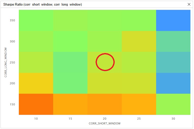
The red circle in the preceding image identifies the parameters we chose as the strategy's default. We chose a short-term correlation window of 20 and a long-term correlation window of 250 because those were the values used in the source paper. However, these defaults are not the combination we found to maximize the risk-adjusted returns. The highest Sharpe ratio in the grid sits at a short-term correlation window of 10 and a long-term correlation window of 150, in the lower-left corner of the tested range.
The long-term correlation window is the more systematic of the two parameters. Holding the short window fixed, the Sharpe ratio generally declines as the long-term window lengthens, with the steepest drop between 150 and 200 days and a flat plateau beyond 250 days. The short-term window matters most at its extremes. A short-term window of 10 days is consistently strong, values from 15 to 25 days cluster close together, and 30 days is the weakest column across nearly every long window. Both parameters reach their best values at the lower edge of the grid, so the in-sample optimum sits on the boundary. Because the windows gate only the short leg, this preference likely reflects how quickly the hedge engages in a fast drawdown. In March 2020, only the shortest windows had the short leg on while the 250 and 350-day windows sat out the decline, although the advantage rests on a handful of such episodes and is not statistically decisive.
Across the grid, the strategy beat the benchmark in 24 of 25 configurations, so its edge over buy-and-hold does not hinge on a single lucky parameter choice. The sensitivity surface is mild, with Sharpe ratios spanning roughly 0.40 to 0.57 and a mean near 0.49. The boundary optimum suggests a follow-up search over shorter correlation windows could lift in-sample Sharpe further, although the paper's 20 and 250-day windows already land near the center of the performance range. Future work could also sweep the short weight and the number of long ETFs, which this research held constant.
References
- Pauchlyová, M., & Vojtko, R. (2025). Refining ETF Asset Momentum Strategy. Quantpedia. SSRN. https://ssrn.com/abstract=5095447


Derek Melchin
The material on this website is provided for informational purposes only and does not constitute an offer to sell, a solicitation to buy, or a recommendation or endorsement for any security or strategy, nor does it constitute an offer to provide investment advisory services by QuantConnect. In addition, the material offers no opinion with respect to the suitability of any security or specific investment. QuantConnect makes no guarantees as to the accuracy or completeness of the views expressed in the website. The views are subject to change, and may have become unreliable for various reasons, including changes in market conditions or economic circumstances. All investments involve risk, including loss of principal. You should consult with an investment professional before making any investment decisions.
To unlock posting to the community forums please complete at least 30% of Boot Camp.
You can continue your Boot Camp training progress from the terminal. We hope to see you in the community soon!