Dual-MA Trend with Volatility Targeting on CSI 300 ETF: Portability, Not Alpha

Dual-MA Trend with Volatility Targeting on CSI 300 ETF: Portability, Not Alpha

A concise and informative title that reflects the main focus of the research. (use the line above as the Title field)

Introduction

Simple moving-average crossovers are among the oldest documented trading rules (Brock, Lakonishok, and LeBaron 1992). In an equity-index setting they are a blunt implementation of time-series momentum (Moskowitz, Ooi, and Pedersen 2012). This note asks a narrower, more practical question: can the same dual-MA rule, once risk-scaled, be reproduced on three execution engines without look-ahead, and what residual return difference is then left to data and fill conventions?

The asset is the Shanghai-listed CSI 300 ETF 510300. The economic claim is drawdown compression, not excess compound return versus buy-and-hold. Two overlays sit on top of a slow SMA cross: an ATR trend-strength filter, and 12% volatility targeting with a 10% weight grid and a leverage cap of one (Moreira and Muir 2017; Barroso and Santa-Clara 2015). Parameters are frozen on 2019–2022; 2023 onward is reported, not retuned.

A Lean backtest of the identical specification on QuantConnect Cloud, using the same static-qfq CSV as custom data, produced a 15.62% total return and $3,847 in fees versus 15.09% and 3,607 on the local event-driven engine. The path is portable. QuantConnect has no native SSE live tape, so the exercise proves logic portability, not Shanghai call-auction fills.

Public Lean result: Determined Orange Jaguar.
Specification and local research: event-driven-backtest-engine.

Method

Universe and sample. Daily OHLCV for 510300, static forward adjustment (qfq), 2019-01-01 through the last available bar (local: 2026-08-25; Lean custom data ended 2026-05-29). Initial capital 1,000,000. Halt bars (volume = 0) remain in the moving-average window but do not fill.

Signal (after the close of day T). Let P_t be the adjusted close.

\mathrm{SMA}{30} and \mathrm{SMA}{120} on close (simple, not exponential).

\mathrm{TR}t = \max(H_t-L_t, |H_t-P{t-1}|, |L_t-P_{t-1}|); ATR is the 20-day mean of TR.

In-trend iff \mathrm{SMA}{30} > \mathrm{SMA}{120} and (\mathrm{SMA}{30}-\mathrm{SMA}{120})/\mathrm{ATR}_{20} > 1.

Realized vol \sigma_t is the 20-day population standard deviation of close-to-close returns, annualized with \sqrt{252}.

Target weight w_t = \mathrm{round}_{0.1}\big(\min(1, 0.12/\sigma_t)\big) when in-trend, else 0.

Execution. w_t is known only after T’s close. The first fill is T+1 open, lot size 100. Commission 1 bp (floor 0.1), transfer 0.1 bp, no stamp tax, 5 bp slippage. No daily drift rebalance: tickets fire only when the rounded weight changes.

Design against look-ahead. On Lean, OnData stores yesterday’s weight and trades today’s Open. Immediate-fill on the signal bar is treated as look-ahead. Custom data uses NullBuyingPowerModel plus a 2% cash buffer so QC’s default margin model does not silently skip rebalances (that failure produced a spurious 2026 spike in an earlier run). Fee and slippage models are attached in SetSecurityInitializer; custom data otherwise defaults to zero fees.

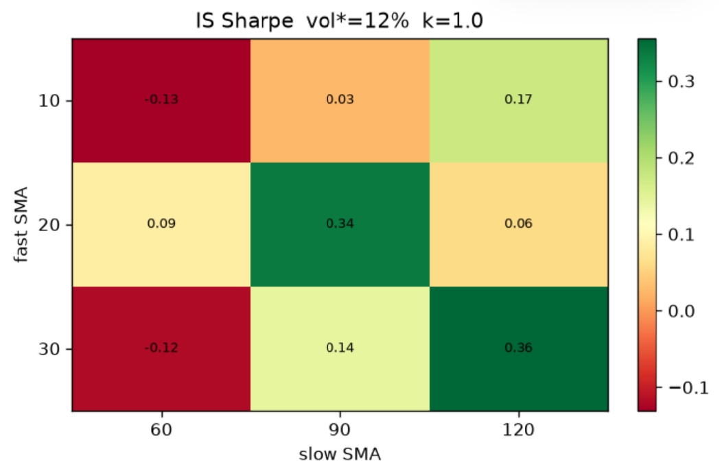
Parameter selection. Grid on the in-sample window only: fast ∈ {10,20,30}, slow ∈ {60,90,120}, vol* ∈ {8%,10%,12%}, k ∈ {0, 0.5, 1.0}. Selection: maximum IS Sharpe among configs with max drawdown ≥ −40%. Winner: SMA 30/120, k=1, vol target 12%. Out-of-sample is not used to pick windows.

Controls. Buy-and-hold 510300 on the same panel, same costs. Cross-engine ablation (fill timing, fee schedule, Sharpe convention) is run on the local engine with one change per run.

Lean implementation. PythonData class Csi300Etf streams
https://raw.githubusercontent.com/david-quant-logs/event-driven-backtest-engine/main/platforms/quantconnect/data/510300.csv.

Results

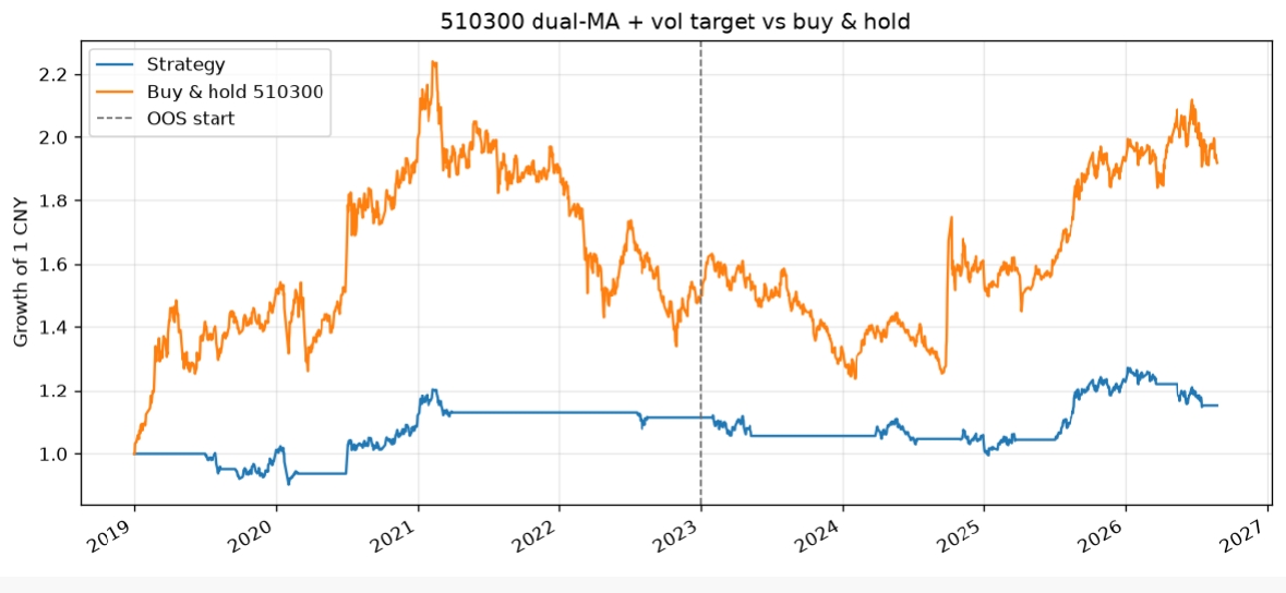
Local engine versus buy-and-hold

OOS Sharpe (0.339) is essentially unchanged from IS (0.356). Compounded return loses to buy-and-hold in both windows; peak-to-trough loss is about one-third of the ETF. Full-sample fees are 3,607 on 173 tickets.

(Insert figures: growth-of-1 versus buy-and-hold; IS Sharpe heatmap at vol = 12% and k = 1.)*

QuantConnect Cloud (same CSV, same rule)

Shared backtest Determined Orange Jaguar, 2019-01-01 to 2026-05-29, cash 1,000,000, Lean 2.5.0.0.18036:

Link: https://www.quantconnect.cloud/backtest/97782a6933f5ad26546e921833bcb2e3/?theme=darkly

An earlier Cloud run reported $0 fees and insufficient buying power from 2019-10-25, with a five-year flat equity curve then a 2026 spike. That run is discarded. After the security initializer and cash cap, fees and the equity path line up with the local engine.

Ablations (local engine, one change at a time)

Relative to the 1.93% local CAGR baseline:

Signal used at T’s open (one day early): +0.38 pp CAGR, Sharpe 0.258 → 0.318 (look-ahead).

T+1 close fills instead of T+1 open: −0.31 pp.

JoinQuant stock default fees (3 bp + stamp tax) instead of ETF fund fees: −0.30 pp, fees 26,350.

IB-like ~12.5 bp on a ~4 CNY price: −0.48 pp, fees 40,251.

Same equity, Sharpe with rf = 2%: 0.258 → 0.035.

Halt-day conventions: 0.00 pp on this ETF (zero halt bars in sample).

Discussion

The results answer the research question in two parts.

First, the overlay does what it is specified to do. It does not beat CSI 300 on compound return. It cuts drawdown from −44.8% to −17.4% in sample and keeps OOS Sharpe stable. That is consistent with volatility-managed momentum: you sell some of the right tail to buy a smaller left tail (Moreira and Muir 2017). The failure mode is a long, low-vol grind higher with shallow pullbacks—the filter stays partly in cash and the slow SMA misses the first month of each leg. 2021–2022 and 2023–2024 chop is where the sleeve earns its keep.

Second, engine residuals are small once defaults are overridden. A 0.5 pp gap in total return between Lean and the local book is the order of fill-timestamp and sample-end differences, not a different strategy. Un-overridden QC IB fees or JoinQuant stock commissions would have moved CAGR by −0.3 to −0.5 pp—larger than the remaining Lean residual. The one-day-early fill is the most dangerous “improvement”: it inflates Sharpe by 0.06 and is not tradable in a cash ETF.

Limitations. (1) QuantConnect Cloud has no SSE live feed; custom daily CSV is not a call auction. Paper trading on a Free organization has zero live nodes and was not deployed. (2) Vendor adj_factor is identically 1 on this file, so static versus dynamic qfq cannot be split on 510300; the one-day signal shift is only a proxy. (3) A single liquid ETF is not a cross-section. (4) QuantConnect PSR on this backtest is ~0.08%, which is the platform’s verdict on a 0.26 Sharpe sleeve—not a reason to reopen the grid.

Future work. Repeat the same spec on a US liquid ETF (SPY) with native Lean data; add a 10% rebalance band versus the current 10% round; compare JoinQuant dynamic qfq on names with actual dividends.

Conclusion

A 30/120 SMA trend, ATR strength filter k=1, and 12% vol targeting on 510300 is a portable risk sleeve, not an alpha product. In-sample and out-of-sample Sharpes match; buy-and-hold still wins on CAGR; drawdown is compressed to about one-third. The same rule on QuantConnect custom data reproduces local total return to within half a percentage point after attaching an A-share ETF fee model and disabling bogus margin rejects.

Recommendation: publish the Lean clone and the specification, not a retuned window. If a platform’s headline return diverges by more than ~1 pp, check fill timing and the default fee schedule before touching fast/slow.

References

• Barroso, P., and P. Santa-Clara. 2015. “Momentum Has Its Moments.” Journal of Financial Economics 116 (1): 111–120.
• Brock, W., J. Lakonishok, and B. LeBaron. 1992. “Simple Technical Trading Rules and the Stochastic Properties of Stock Returns.” Journal of Finance 47 (5): 1731–1764.
• Moreira, A., and T. Muir. 2017. “Volatility-Managed Portfolios.” Journal of Finance 72 (4): 1611–1644.
• Moskowitz, T. J., Y. H. Ooi, and L. H. Pedersen. 2012. “Time Series Momentum.” Journal of Financial Economics 104 (2): 228–250.

Public backtest:

https://www.quantconnect.cloud/backtest/97782a6933f5ad26546e921833bcb2e3/?theme=darkly

Code and spec: https://github.com/david-quant-logs/event-driven-backtest-engine