


 Share New Research


Introduction
Most momentum strategies rank stocks and buy a fixed number of the strongest, which forces the portfolio to hold that many stocks, regardless of how many of them are genuinely exceptional. The strategy in this research post lets the cross-section decide the portfolio size by selecting only statistical outliers. Each day, it selects the US Equities with their dollar volume more than two standard deviations above the cross-sectional mean. It then applies the same test to momentum among the survivors. Winsorized statistics keep those thresholds stable, and the portfolio holds however many stocks clear both bars, equally weighted, rebalanced every morning. From September 2021 to September 2026, the strategy achieved a 0.525 Sharpe ratio, outperforming the 0.363 Sharpe ratio for a buy-and-hold position in the SPY.
Background
Jegadeesh and Titman (1993) documented momentum by ranking stocks on their past returns and holding the top decile. Most implementations since have kept a fixed-count construction, whether the top decile, the top quintile, or the top \( n \), so the selectivity of the portfolio never responds to how unusual the strongest stocks actually are. An alternative statistically defines membership, admitting a stock only while its factor value sits more than a fixed number of standard deviations above the cross-sectional mean. When the market offers a fat tail of exceptional stocks, the portfolio widens to hold them, and when the cross-section is unremarkable, the portfolio narrows to the few stocks that still stand out.
Setting an outlier threshold from raw cross-sectional moments fails in practice because the same extreme observations the strategy hunts also inflate the mean and standard deviation that define the threshold. For instance, a small number of mega-cap stocks dominate the dollar-volume cross-section and a few meme-stock moves can double the dispersion of momentum. The standard remedy is winsorization, which caps the most extreme values in both tails before the moments are measured, giving the threshold
\[ T = \mu_w + 2\sigma_w, \]
where \( \mu_w \) and \( \sigma_w \) are the mean and standard deviation of the winsorized values. Each stock's raw, unclipped value is then compared against \( T \), so the threshold is robust to outliers while the selection still rewards them.
The first pass of the outlier test selects the stocks that have their average daily dollar volume over the lookback window above the threshold, concentrating the universe in the most heavily traded stocks. The second pass applies the same test to momentum over the same window among those liquid stocks. Survivors enter an equal-weighted portfolio that rebalances every morning, so membership lasts exactly as long as a stock remains exceptional on both dimensions.
Implementation
To implement this strategy, we start by defining the parameters and adding a universe of US Equities in the initialize method.
# Define some parameters
self._period = 9 * 21
self._winsor_percentile = 5.0
self._std_multiplier = 2
# Add an universe of US Equities based on indicators.
self._selection_data_by_symbol = {}
self.universe_settings.resolution = Resolution.DAILY
self._universe = self.add_universe(self._select_assets)
At the end of the initialize method, we add a Scheduled Event that rebalances the portfolio at each market open.
self.schedule.on(self.date_rules.every_day('SPY'), self.time_rules.at(8, 0), self._rebalance)For every stock in the US Equity market, the algorithm maintains a SelectionData object, which tracks the momentum and the average daily dollar volume over the lookback window.
class SelectionData:

    def __init__(self, period):
        self.momentum = MomentumPercent(period)
        self.mean_dollar_volume = SimpleMovingAverage(period)

    def update(self, f):
        return (
            self.momentum.update(f.end_time, f.adjusted_price) &
            self.mean_dollar_volume.update(f.end_time, f.dollar_volume)
        )
Each day, the _select_assets universe selection function first updates every stock's indicators and collects the stocks whose indicators are ready.
def _select_assets(self, fundamentals: List[Fundamental]):
    candidates = []
    for f in fundamentals:
        if not f.has_fundamental_data:
            continue
        if f.symbol not in self._selection_data_by_symbol:
            self._selection_data_by_symbol[f.symbol] = SelectionData(self._period)
        if self._selection_data_by_symbol[f.symbol].update(f):
            candidates.append(f.symbol)
The method then applies the outlier test twice, first to average dollar volume and then to momentum among the survivors, so the universe holds the momentum outliers of the liquidity outliers.
candidates = self._outliers(candidates, lambda s: self._selection_data_by_symbol[s].mean_dollar_volume.current.value)
return self._outliers(candidates, lambda s: self._selection_data_by_symbol[s].momentum.current.value)
Both calls go through the _outliers method, which computes the winsorized threshold for any factor and returns the stocks with raw values above it.
def _outliers(self, candidates, factor):
    values = np.array([factor(s) for s in candidates])
    # Winsorize the values so extreme outliers don't skew the standard deviation calculation.
    lower, upper = np.percentile(values, [self._winsor_percentile, 100 - self._winsor_percentile])
    clipped = np.clip(values, lower, upper)
    # Calculate the threshold based on standard deviations.
    threshold = clipped.mean() + self._std_multiplier * clipped.std()
    # Select the stocks that exceed the threshold.
    return [candidates[i] for i in np.where(values > threshold)[0]]
Finally, the _rebalance method forms an equal-weighted portfolio of the current universe constituents, liquidating the positions that left the selection.
def _rebalance(self):
    # During warm-up, do nothing.
    if self.is_warming_up:
        return
    # Form an equal-weighted portfolio.
    weight = 1.0 / len(self._universe.selected)
    self.set_holdings([PortfolioTarget(s, weight) for s in self._universe.selected ], liquidate_existing_holdings=True)
Results
We backtested the strategy from September 2021 to September 2026. Over that period the strategy earned a 0.525 Sharpe ratio. In contrast, a buy-and-hold position in the SPY over the same time period achieved a 0.363 Sharpe ratio. Therefore, the strategy outperformed the benchmark.
We ran a parameter optimization job to test the sensitivity of the chosen parameters. We tested the lookback in months from 6 to 12 in steps of 1, and we tested the winsorization percentile from 2.5 to 7.5 in steps of 1. Of the 42 parameter combinations, 42/42 (100%) produced a greater Sharpe ratio than the benchmark. The following image shows the heatmap of Sharpe ratios for the parameter combinations:
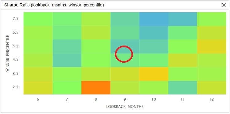
The red circle in the preceding image identifies the parameters we chose as the strategy's default. We chose a nine-month lookback from the middle of the standard six-to-twelve-month momentum formation range, and a winsorization percentile of 5 because clipping at the 5th and 95th percentiles is the most common winsorization convention in empirical asset pricing. The percentile default sits between two tested columns, whose lookback-9 cells produced Sharpe ratios of 0.531 and 0.483, close to the 0.525 the default parameters earned in the full backtest.
Every one of the 42 tested combinations beat the benchmark, with Sharpe ratios spanning 0.444 to 0.807. Within that band the surface is jagged rather than trending, with neither parameter moving the Sharpe ratio in a consistent direction. The largest swings sit in the 2.5-percentile column (0.504 to 0.807), and the best tested combination, an eight-month lookback with a 2.5 winsorization percentile, sits at the edge of the tested percentile range while its immediate lookback neighbors produced 0.574 and 0.633. Differences of this size are well within the estimation uncertainty of a Sharpe ratio measured over a five-year sample, so we read the variation inside the band as sample noise rather than structure, and we do not treat the peak cell as a better default.
Future research could add a floor or cap on the number of holdings to control the concentration risk that comes with a floating portfolio size. It could also weight each holding by its distance above the threshold rather than equally, so the most exceptional stocks carry the most capital. A short leg built from the lower tail of the momentum cross-section would extend the design to the long-short form of Jegadeesh and Titman (1993).
References
- Jegadeesh, N., & Titman, S. (1993). Returns to Buying Winners and Selling Losers: Implications for Stock Market Efficiency. The Journal of Finance, 48(1), 65-91.


Derek Melchin
The material on this website is provided for informational purposes only and does not constitute an offer to sell, a solicitation to buy, or a recommendation or endorsement for any security or strategy, nor does it constitute an offer to provide investment advisory services by QuantConnect. In addition, the material offers no opinion with respect to the suitability of any security or specific investment. QuantConnect makes no guarantees as to the accuracy or completeness of the views expressed in the website. The views are subject to change, and may have become unreliable for various reasons, including changes in market conditions or economic circumstances. All investments involve risk, including loss of principal. You should consult with an investment professional before making any investment decisions.
To unlock posting to the community forums please complete at least 30% of Boot Camp.
You can continue your Boot Camp training progress from the terminal. We hope to see you in the community soon!