


 Share New Research


Introduction
Algorithmic execution leaves a fingerprint on the tape. When many participants slice parent orders on regular schedules, intraday trading volume develops persistent high-frequency periodicities that a spectral decomposition can measure. Wu, Zhang and Dai (2025) document these periodicities across the US and Chinese markets and show they carry information about price formation. This post builds a US Equity, long-only, cross-sectional strategy on that idea. Each week, the algorithm ranks the 100 most liquid US Equities by the strength of their intraday-volume periodicity, selects the top quintile of stocks, and tilts the weights toward the stocks with the strongest execution flow. These factors are provided by our new Spectral Tick-Flow Signal dataset. The results show that the algorithm outperformed the buy-and-hold benchmark over the last 5 years.
Background
Trading volume is not spread evenly across the trading day. Beyond the familiar U-shaped pattern of heavy volume near the open and the close, the intraday volume series repeats at much shorter horizons, on the order of seconds to minutes. Wu et al. (2025) attribute this regularity to execution algorithms that release child orders at fixed intervals, and they measure it with a spectral decomposition of the intraday volume series. Decomposing volume into its frequency components isolates a dominant period, the interval at which the pattern repeats, along with the share of total intraday volume variance that this dominant frequency explains. The larger that share, the more mechanically periodic the stock's trading is that day.
Intraday Volume Periodicity
The Spectral Tick-Flow Signal dataset publishes both quantities for each liquid US Equity every trading day. The dominant period arrives as volume_dominant_period_seconds, and the normalized strength of the pattern arrives as volume_variance_explained, a figure that rises toward one as a single intraday frequency comes to dominate the volume series. We treat volume_variance_explained as the periodicity score, mirroring the paper's own measure, which summarizes the fraction of de-trended intraday volume variance explained by the strongest periodic terms. Wu et al. (2025) find that future returns correlate with periodicity score because of information asymmetry. Periodic trading carries more information content, so investors face greater adverse selection and demand a higher return to hold the most periodic stocks.
Execution-Flow Confirmation
The Spectral Tick-Flow Signal dataset carries a second, independent read on the tape. Alongside the volume-flow track, an execution-flow track scores how strong and how regular a stock's execution program is, exposed as execution_score. A high execution score means the periodicity is backed by an active, repeating execution signature rather than an incidental volume artifact. We use the execution score in this research not as a filter but as a weighting signal, tilting more capital toward the stocks whose periodicity is most strongly confirmed by execution flow.
Position Sizing
To keep the tilt stable from week to week, we smooth each stock's execution score into a persistent execution intensity. The intensity is an exponentially-weighted moving average of the daily execution score. We then assign a raw weight to each stock
\[ r_i = 1 + \frac{e_i}{\max_j e_j}, \]
where \( e_i \) is stock \(i\)'s persistent execution intensity and \( \max_j e_j \) is the largest execution intensity across the stocks. This way, a stock's weight in the portfolio grows with its intensity relative to the strongest one. The additive one guarantees every stock keeps a baseline allocation when its execution intensity is near zero, and it bounds each raw weight to the interval \([1, 2]\). Normalizing the raw weights produces the final portfolio weight
\[ w_i = \frac{r_i}{\sum_j r_j}, \]
where the denominator sums the raw weights across the long leg so the portfolio stays fully invested.
Implementation
To implement this strategy, we start by adding a universe of the 100 most liquid US Equities. Each week, the algorithm selects the 100 stocks with the highest dollar volume, which keeps the universe in the large, liquid stocks where the periodicity premium lives.
self.universe_settings.resolution = Resolution.DAILY
self._date_rule = self.date_rules.week_start("SPY")
self.universe_settings.schedule.on(self._date_rule)
self._universe = self.add_universe(lambda fundamental:
   [f.symbol for f in sorted([f for f in fundamental if f.has_fundamental_data], key=lambda f: f.dollar_volume)[-100:]]
)
As stocks enter the universe, we add the Spectral Tick Flow Signal dataset for each one and create an exponential moving average of its execution-flow signal over the trailing three months. We warm up the EMA from history so the stock is ready to trade at the next rebalance.
for security in changes.added_securities:
    security.dataset_symbol = self.add_data(QuantConnectSpectralTickFlowSignal, security, Resolution.DAILY).symbol
    security.exec_intensity = ExponentialMovingAverage(self._ema_period)
    for data_point in self.history[QuantConnectSpectralTickFlowSignal](security.dataset_symbol, timedelta(int(self._ema_period*1.5))):
        self._update_factors(security, data_point)
The _update_factors helper method stores the latest signal and updates the execution-intensity average. It runs both while seeding from history and in on_data as new daily signals arrive.
def _update_factors(self, security: Equity, data_point: QuantConnectSpectralTickFlowSignal) -> None:
    security.signal = data_point
    security.exec_intensity.update(data_point.end_time, data_point.execution_score)
Once warm-up finishes, we add a Scheduled Event to rebalance the portfolio at the start of each week at 8 AM Eastern Time (ET). Universe selection runs between 7 and 8 AM ET in live trading, so firing at 8 AM guarantees the rebalance sees the current week's constituents.
time_rule = self.time_rules.at(8, 0)
self.schedule.on(self._date_rule, time_rule, self._rebalance)
Inside the _rebalance method, we take the current universe constituents whose execution-intensity average is ready, then keep the top quintile ranked by the strength of their volume periodicity.
securities = [self.securities[symbol] for symbol in self._universe.selected]
eligible = [security for security in securities if security.exec_intensity.is_ready]
selected = sorted(eligible, key=lambda security: security.signal.volume_variance_explained)[-int(len(eligible)/self._quantiles):]
We then give each selected stock a raw weight of one plus its execution intensity relative to the strongest stock in the group, which tilts exposure toward the most intensely algo-executed stocks without dropping the rest. Normalizing the raw weights leaves the portfolio fully invested and long-only. The algorithm rebalances to these portfolio targets and liquidates any holding that left the selection.
peak = max((security.exec_intensity.current.value for security in selected))
weight_by_security = {security: 1.0 + security.exec_intensity.current.value / peak for security in selected}
weight_by_security = {security: weight / sum(weight_by_security.values()) for security, weight in weight_by_security.items()}
targets = [PortfolioTarget(security, weight) for security, weight in weight_by_security.items()]
self.set_holdings(targets, True)
Results
We backtested the strategy over July 2021 to July 2026. Over that period, the strategy earned a 0.792 Sharpe ratio. In contrast, a buy-and-hold position in the SPY over the same time period achieved a 0.406 Sharpe ratio. Therefore, the strategy outperformed the benchmark.
We ran a parameter optimization job to test the sensitivity of the chosen parameters. We varied the universe size from 50 to 150 stocks in steps of 25, and we varied the execution-intensity EMA length from 1 to 5 months in steps of 1 month. Of the 25 parameter combinations, all 25 (100%) produced a greater Sharpe ratio than the benchmark. The following image shows the heatmap of Sharpe ratios for the parameter combinations:
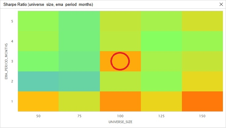
The red circle in the preceding image identifies the parameters we chose as the strategy's default. We chose a universe size of 100 stocks and a 3-month execution-intensity EMA because the 100-stock universe delivers the strongest average Sharpe ratio across the five EMA lengths and a 3-month average smooths the execution-intensity signal more than the fast 1-month setting. These defaults are not the Sharpe-maximizing combination. The highest Sharpe ratio in the grid sits at a universe size of 150 and a 1-month EMA, in the corner of the tested range. However, an optimum pinned to the edge of the search range is more likely an artifact of where the search stops than a stable choice.
The EMA length is the more sensitive of the two parameters. A 1-month EMA is uniformly the strongest setting, and the Sharpe ratio drops sharply when the length increases from 1 to 2 months at every universe size. Beyond 2 months the surface is choppy with no clear trend. The universe size matters less and its response is rugged, though larger universes generally help. The 100 and 150-stock columns are the strongest and 75 stocks is the weakest. Both parameters reach their joint best value at the edge of the grid, the largest universe paired with the shortest EMA, so the in-sample optimum sits on the boundary.
Across the grid, the strategy beat the benchmark in all 25 configurations, so its edge over buy-and-hold does not depend on the exact parameter choice. Sharpe ratios span roughly 0.57 to 0.83 with a mean near 0.68. The dominance of the short-EMA region suggests the execution-intensity signal is most useful when it reacts quickly. The boundary optimum points to further research on a universe larger than 150 stocks and on sub-monthly EMA lengths, both of which may increase the in-sample Sharpe ratio further.
References
- Wu, L., Zhang, R., & Dai, Y. (2025). Spectral Volume Models: Universal High-Frequency Periodicities in Intraday Trading Activities. SSRN.


Rudy Osuna
The material on this website is provided for informational purposes only and does not constitute an offer to sell, a solicitation to buy, or a recommendation or endorsement for any security or strategy, nor does it constitute an offer to provide investment advisory services by QuantConnect. In addition, the material offers no opinion with respect to the suitability of any security or specific investment. QuantConnect makes no guarantees as to the accuracy or completeness of the views expressed in the website. The views are subject to change, and may have become unreliable for various reasons, including changes in market conditions or economic circumstances. All investments involve risk, including loss of principal. You should consult with an investment professional before making any investment decisions.
To unlock posting to the community forums please complete at least 30% of Boot Camp.
You can continue your Boot Camp training progress from the terminal. We hope to see you in the community soon!