


Abstract
In this tutorial we build a strategy combining momentum and mean reversion for the foreign exchange markets from Alina F. Serban's research which was based on research in the equity market by Ronald J. Balvers and Yangru Wu. Serban creates a momentum factor using returns of the last 3 months, and a mean reversion factor as a deviation from the mean price. Using these factors we use regression to predict the returns of the coming month. We apply the strategy from Serban's paper and update the mean reversion factor to improve its significance level.
In theory when trading foreign exchange the expected return accrued in each currency should be the same when adjusted for exchange rates (uncovered interest parity). This suggests the markets should predominately be mean reverting, however in practice we see short term momentum trends and long term mean reversion. This was phenomenon was first noticed by Chiang and Jiang. We tested the theory on EURUSD, GBPUSD, USDCAD and USDJPY and re-balanced monthly. The model significance level and coefficients are close to those in paper, but the returns and Sharpe Ratios obtained are not as good as what the paper claimed. The algorithm achieved a fairly stable annual return of 11%, 0.8 Sharpe Ratio and 11% drawdown.
Introduction
The strategy is centered on uncovered interest parity (UIP) theory. UIP states that the change in the exchange rate should incorporate any interest rate differentials between the two currencies. By looking for patterns in the deviation from UIP we can potential generate abnormal returns.
Interest Parity Conditions
UIP states that an investor who borrows money in their home country and lends it in another country with a higher interest rate should expect a zero return due to the changes in exchange rate. In other words:
\[1+r_t = (1+r^{i}_t)\left(\frac{F^{i}_t}{S^{i}_t}\right)\]
where \(r_t\) is the domestic interest rate, \(r^{i}\) is the foreign interest rate, \(S^{i}\) is the spot exchange rate, and \(F^{i}\) is the forward rate. We can also replace the forward rate with the expected spot rate:
\[1+r_t = (1+r^{i}_t)\left(\frac{E(S^{i}_{t+1})}{S^{i}_t}\right)\]
Taking logs of the above two equations, we obtain:
\[r_t - r^{i}_t = \ln F^{i}_t - \ln S^{i}_t\]
\[r_t - r^{i}_t =\ln S^{i}_{t+1} - \ln S^{i}_t\]
The deviation from UIP is denoted by \(y\) and defined as follows:
\[y^{i}_{t+1} =\ln S^{i}_{t+1} -\ln F^{i}_t\]
Model and Parameter Estimation
Fama and French and Summers constructed a simple model for stock price that is the sum of a random walk and a stationary component - they represent the natural log of the stock price with \(x\). The stationary component represents the temporary swings in stock price (characterized by coefficient \(\delta \)), the parameter \(\mu \) captures the random walk drift component and a coefficient accounts for the momentum effect \(\rho\). Balvers and Wu construct the log of stock prices as:
\[\begin{equation} \begin{aligned} x^{i}_t = \ & (1 - \delta ^{i})\mu ^{i} + \delta ^{i}x^{i}_{t-1} \\ & + \sum_{j=1}^{J}\rho ^{i}(x^{i}_{t-1} - x^{i}_{t-j-1}) + \epsilon ^{u}_t \end{aligned} \end{equation}\]
Using the equation above Serban adapts it to find the abnormal return in the forex market. The \(\delta \) represents the speed of mean reversion and can differ by country, while the \(\rho \) represents the momentum strength and can vary by country and by lag. The parameter \(\mu \) also varies by country. Accounting for these changes:
\[\begin{equation} \begin{aligned} y^{i}_t = \ & -(1 - \delta ^{i})(x^{i}_{t-1} - \mu ^{i}) \\ & + \sum_{j=1}^{J}\rho ^{i}(x^{i}_{t-1} - x^{i}_{t-j-1}) + \epsilon ^{u}_t \end{aligned} \end{equation}\]
Trading Strategy
The trading strategy from the paper allows \(\mu \) to change by country, while let \(\rho \) and \(\delta \) stay fixed. By applying Ordinary Least Squared (OLS) regression, the model estimates the return \(y\) for each currency. We construct the portfolio by taking a long position on the currency with the highest expected return and taking a short position on the currency with the lowest expected return. We hold these positions for one month, and repeat the process each month. There are two exceptions to this strategy: if all expected returns are positive, we take a long position only, and vice versa. To limit the number of parameters we need to estimate and find a solution easily we only allow \(\mu \) to change by country. According to the paper if we let \(ρ\) stay fixed and \(J=3\), we can obtain the highest return for this strategy. If so the equation can be simplified as:
\[\begin{equation} \begin{aligned} y^{i}_t = \ & -(1-\delta )(x^{i}_{t-1} - \mu ^{i}) \\ & + \rho (x^{i}_{t-1} - x^{i}_{t-4}) + \epsilon ^{i}_t \end{aligned} \end{equation}\]
When applying the above equation, we found that the scale of the mean reversion for each currency are very different, and this difference in scale is large enough to affect the accuracy of our rank. We made an adjustment to standardize the mean-reversion. While calculating \(\mu \) (the mean of the log prices) we also calculated standard deviation \(σ\). In this tutorial, we replace \(x-\mu \) with \(\frac{x - \mu}{\sigma } \). This captures the mean reversion factor better than the author's technique.
Data Description
The paper used monthly exchange rate data for the Canadian Dollar/USD, German Mark/Euro, UK Pound/USD and Japanese Yen/USD, from 1978 to 2008. Due to data availability, we used Euro/USD instead of German Mark/Euro, and the earliest data available starts from 2004. Each time we launch the strategy we use all of the available historical data prior to the start date to build the OLS model and use that model for the entire backtest. The paper used 1/3 of their data as the training dataset and the rest of the test set. We directly test our model on backtesting, because QuantConnect makes this easier.
Method
In order to apply the model, we need to first pull historical data to build it. The project can be briefly divided into four parts: the historical data request, model training, prediction and execution.
Step 1: Request Historical Data
The first function takes two arguments: symbol and number of daily data points requested. This function requests historical data and builds it into a pandas DataFrame. For more information about the pandas DataFrame, see the reference on the Pydata website. The calculate_return function takes a DataFrame as an argument to calculate the mean and standard deviation of the log prices, and create new columns for the DataFrame (return, reversal factor and momentum) - it prepares the DataFrame for multiple linear regression.
def get_history(self,symbol, num):
    data = {}
    dates = []
    history = self.history([symbol], num, Resolution.DAILY).loc[symbol]['close'] #request the historical data for a single symbol
    for time in history.index:
        t = time.to_pydatetime().date()
        dates.append(t)
    dates = pd.to_datetime(dates)
    df = pd.DataFrame(history)
    df.reset_index(drop=True)
    df.index = dates
    df.columns = ['price']
    return df

def calculate_return(self,df):
    #calculate the mean for further use
    mean = np.mean(df.price)
    # cauculate the standard deviation
    sd = np.std(df.price)
    # pandas method to take the last datapoint of each month.
    df = df.resample('BM').last()
    # the following three lines are for further experiment purpose
    # df['j1'] = df.price.shift(1) - df.price.shift(2)
    # df['j2'] = df.price.shift(2) - df.price.shift(3)
    # df['j3'] = df.price.shift(3) - df.price.shift(4)
    # take the return as depend variable
    df['log_return'] = df.price - df.price.shift(1)
    # calculate the reversal factor
    df['reversal'] = (df.price.shift(1) - mean)/sd
    # calculate the momentum factor
    df['mom'] = df.price.shift(1) - df.price.shift(4)
    df = df.dropna() #remove nan value
    return (df,mean,sd)
Step 2: Build Predictive Model
The concat function requests history and joins the results into a single DataFrame. As \(\mu\) varies by country so we assign the mean and standard deviation to the symbol for each currency for future use. The OLS function takes the resulting DataFrame to conduct an OLS regression. We write it into a function because it's easier to change the formula here if we need.
def concat(self):
    # we requested as many daily tradebars as we can
    his = self.get_history(self.quoted[0].value,20*365)
    # get the clean DataFrame for linear regression
    his = self.calculate_return(his)
    # add property to the symbol object for further use.
    self.quoted[0].mean = his[1]
    self.quoted[0].sd = his[2]
    df = his[0]
    # repeat the above procedure for each symbols, and concat the dataframes
    for i in range(1,len(self.quoted)):
        his = self.get_history(self.quoted[i].value,20*365)
        his = self.calculate_return(his)
        self.quoted[i].mean = his[1]
        self.quoted[i].sd = his[2]
        df = pd.concat([df,his[0]])
    df = df.sort_index()
    # remove outliers that outside the 99.9% confidence interval
    df = df[df.apply(lambda x: np.abs(x - x.mean()) / x.std() < 3).all(axis=1)]
    return df

def OLS(self,df):
    res = sm.ols(formula = 'return ~ reversal + mom',data = df).fit()
    return res
Step 3: Apply Predictive Model
The predict function uses the history for the last 3 months, merges it into a DataFrame and then calculates the updated factors. Using these updated factors (together with the model we built) we calculate the expected return.
def predict(self,symbol):
    # get current month in string
    month = str(self.time).split(' ')[0][5:7]
    # request the data in the last three months
    res = self.get_history(symbol.value,33*3)
    # pandas method to take the last datapoint of each month
    res = res.resample('BM').last()
    # remove the data points in the current month
    res = res[res.index.month != int(month)]
    # calculate the variables
    res = self.calculate_input(res,symbol.mean,symbol.sd)
    res = res.iloc[0]
    # take the coefficient. The first one will not be used for sum-product because it's the intercept
    params = self.formula.params[1:]
    # calculate the expected return
    re = sum([a*b for a,b in zip(res[1:],params)]) + self.formula.params[0]
    return re

def calculate_input(self, df, mean, sd):
    df['reversal'] = (df.price - mean)/sd
    df['mom'] = df.price - df.price.shift(3)
    df = df.dropna()
    return df
There are a few points of note:
- We need historical TradeBars for the last three months. To do this we requested 99 bars and use a pandas DataFrame to extract a data point for the end of each month.
- We use Scheduled Events to execute the strategy at the first trading day, however, sometimes the first day of the month could be on the 2nd if the 1st falls on a weekend. To fix this we remove the data from the current month, leaving only the last 3 months of data.
- We start from the second element of
res(res[1:]) becauseresandparamsare different lengths. This was hard to detect because Python would not throw error when running[a*b for a,b in zip(res,params)]even if the length of the two lists are different. - This function also used pandas DataFrame methods extensively. For more information about pandas, see the documentation on the Pydata website.
Step 4: Initializing the Model
In the Initialize function, we prepare the data and conduct a linear regression. The class property 'self.formula' is the result of the OLS regression. We will use this object each time we rebalance the portfolio.
def initialize(self):
    self.set_start_date(2013,6,1)
    self.set_end_date(2016,6,1)
    self.set_cash(10000)
    self.syls = ['EURUSD','GBPUSD','USDCAD','USDJPY']
    self.quoted = []
    for i in range(len(self.syls)):
        self.quoted.append(self.add_forex(self.syls[i],Resolution.DAILY,Market.OANDA).symbol)
    df = self.concat()
    self.log(str(df))
    self.formula = self.OLS(df)
    self.log(str(self.formula.summary()))
    self.log(str(df))
    self.log(str(df.describe()))
    for i in self.quoted:
        self.log(str(i.mean) + '   ' + str(i.sd))
    self.schedule.on(self.date_rules.month_start(), self.time_rules.at(9,31), Action(self.action))
Step 5: Performing Monthly Rebalancing
Every month we rebalance the portfolio using the Schedule Event helper method. The predicted returns are added to the rank array and then sorted by return. The first element in the list is the best return paired with the associated symbol. When all the expected returns in the rank array are positive, we only go long the pair with the highest expected return. When all returns are negative, we only go short the pair with the lowest expected return.
def action(self):
    rank = []
    long_short = []
    for i in self.quoted:
        rank.append((i,self.predict(i)))
# rank the symbols by their expected return
    rank.sort(key = lambda x: x[1],reverse = True)
# the first element in long_short is the one with the highest expected return, which we are going to long, and the second one is going to be shorted.
    long_short.append(rank[0])
    long_short.append(rank[-1])
    self.liquidate()

# the product < 0 means the expected return of the first one is positive and that of the second one is negative--we are going to long and short.
    if long_short[0][1]*long_short[1][1] < 0:
        self.set_holdings(long_short[0][0],1)
        self.set_holdings(long_short[1][0],-1)
        # this means we long only because all of the expected return is positive
    elif long_short[0][1] > 0 and long_short[1][1] > 0:
        self.set_holdings(long_short[0][0],1)
# short only
    else:
        self.set_holdings(long_short[1][0],-1)
Results
The following regression output is obtained by backtesting the time period from Jun 2013 to Jun 2016. From the regression statistics, the R-squared value is 1.4%, which is smaller than the paper value 3.89%. Our momentum coefficient, \(ρ\), is 0.0633 compared to the paper's 0.042. We obtained 1.0350 mean reversion coefficient (1 + 0.0350), and the paper got 0.9859.
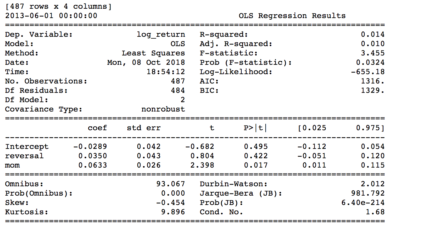
From these results, we can say the limited sample size does not impair the feasibility of this model. The t-stats of the coefficients are -4.074 and 1.417 for the reversal factor and momentum factor respectively. The p-value of the reversal factor is very small which means this factor has a very high significance level.
Backtest Sensitivity Results
We performed some rough period sensitivity analysis in different time period (from 2015 to 2018) and summarized the results as the following table:
| Backtest Period | Annual Return | Sharpe Ratio | Max Drawdown |
|---|---|---|---|
| 2013/06/01-2016/06/01 | -1.938% | -0.056 | 19.800% |
| 2015/06/01-2017/06/01 | -4.008% | -0.171 | 21.700% |
| 2012/06/01-2016/06/01 | -0.958% | -0.013 | 19.700% |
Summary
The paper demonstrates there are inefficiencies in the UIP which can be exploited with a hybrid momentum and mean reversion strategy. Although the sample size of the paper is much larger than ours, the parameter and significance level of the two models are very close. The strategies we discussed above keep \(\rho\) fixed and only allow \(\mu\) to change by country. If we let \(\rho\) change by lag the significance level of the model might increase, but this could potentially make modeling more difficult by introducing multicollinearity. To test this, we wrote this implementation in the algorithm and commented out the lines. If you are interested in exploring this extension to the model you can change these lines to test your strategy.
Reference
- Alina F. Serban, Combining mean reversion and momentum trading strategies in foreign exchange markets Online Copy
- Investopedia, Uncovered Interest Rate Parity. Online Copy
- Ronald J. Balvers, Yangru Wu, Momentum and mean reversion across national equity markets Online Copy
- Chiang, T., Jiang, C., 1995. Foreign exchange returns over short and long horizons. International Review of Economics and Finance 4, 267–282. Online Copy
- Fama, E., 1984. Forward and spot exchange rates. Journal of Monetary Economics 14, 319–338. Online Copy


Derek Melchin
See the attached backtest for an updated version of the algorithm in PEP8 style.
The material on this website is provided for informational purposes only and does not constitute an offer to sell, a solicitation to buy, or a recommendation or endorsement for any security or strategy, nor does it constitute an offer to provide investment advisory services by QuantConnect. In addition, the material offers no opinion with respect to the suitability of any security or specific investment. QuantConnect makes no guarantees as to the accuracy or completeness of the views expressed in the website. The views are subject to change, and may have become unreliable for various reasons, including changes in market conditions or economic circumstances. All investments involve risk, including loss of principal. You should consult with an investment professional before making any investment decisions.
Jing Wu
The material on this website is provided for informational purposes only and does not constitute an offer to sell, a solicitation to buy, or a recommendation or endorsement for any security or strategy, nor does it constitute an offer to provide investment advisory services by QuantConnect. In addition, the material offers no opinion with respect to the suitability of any security or specific investment. QuantConnect makes no guarantees as to the accuracy or completeness of the views expressed in the website. The views are subject to change, and may have become unreliable for various reasons, including changes in market conditions or economic circumstances. All investments involve risk, including loss of principal. You should consult with an investment professional before making any investment decisions.
To unlock posting to the community forums please complete at least 30% of Boot Camp.
You can continue your Boot Camp training progress from the terminal. We hope to see you in the community soon!