


Abstract
In this tutorial, we apply Deep Learning Classification in an attempt to forecast the movement of future stock prices.
Introduction
Various time series forecasting models (SMA, EMA, etc.) have been applied to stocks to forecast price movements. More recently, with the advent of Neural Networks, which have seen applications in several fields, ranging from medicine to fraud detection, researchers have tried to apply Neural Networks to the markets in an attempt to forecast price movements. Convolutional Neural Networks (CNNs) are a class of Neural Networks most widely known for their use in image classification, and now, researchers are applying CNNs to extract patterns, also known as features, from times-series data to forecast future stock prices.
Method
Overview
Our strategy is to develop a Temporal Convolutional Neural Network model and train our model on historical OHLCV data to predict the movement of future prices. Then, when trading, we take the most recent data, feed it into our model, and bet on the direction of the price movement based on our model prediction. We will walk through the code required for building the Neural Network Architecture and for preparing the data for our model, as this part is the harder part to understand.
Inputs/Outputs
Before we build our Neural Network Architecture, we need to understand the inputs and outputs to our model. The input to the model will be the OHLC+Volume data for \(t-14\) to \(t\) time steps (past 15 time steps). The output is a direction (Up, Down, Stationary) of the movement of the average close of the \(t+1\) to \(t+5\) time steps (5 future timestamps). The movement is considered stationary if the abs(% change 5-step average close) < .01%. These three directions will form the labels for which our model will try to classify, thus we have a classification problem.
Neural Network Model Architecture
Now, we will need to build our Neural Network Architecture, which we will build using Keras, a high-level Python Deep Learning API. To begin, we will need a few import statements:
import tensorflow as tf
from tensorflow.keras.layers import Input, Conv1D, Dense, Lambda, Flatten, Concatenate
from tensorflow.keras import Model
from tensorflow.keras import metrics
from tensorflow.keras.losses import CategoricalCrossentropy
from tensorflow.keras import utils
from sklearn.preprocessing import StandardScaler
import numpy as np
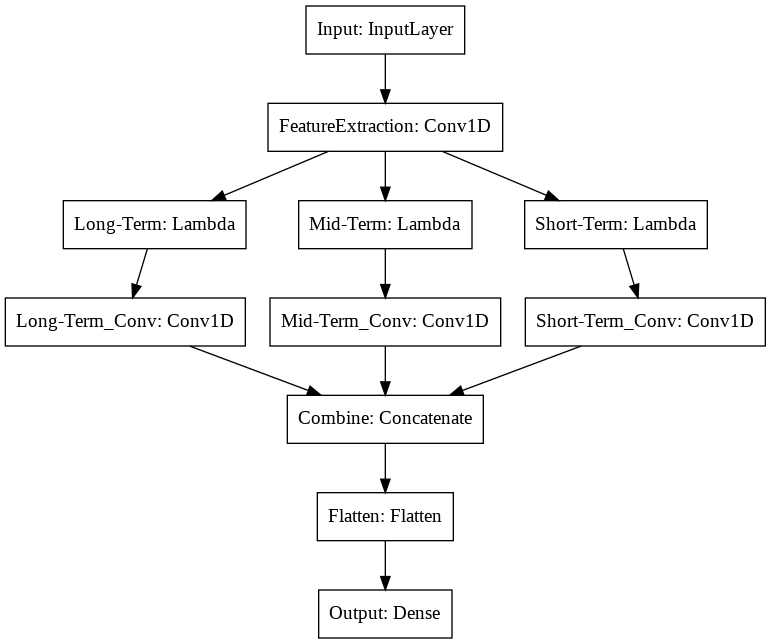
import mathWe start with an Input Layer, where training and testing data are initially accepted. With 15 time steps and 5 input variables (OHLCV), our input shape will be 15 x 5.
inputs = Input(shape=(15, 5))We then feed this Layer into our Convolutional Layer, where we extract features, which will serve as the Neural Network's method of extracting patterns from the time-series data.
feature_extraction = Conv1D(30, 4, activation='relu')(inputs)long_term = Lambda( lambda x: tf.split(x, num_or_size_splits=3, axis=1)[0])(feature_extraction)
mid_term = Lambda( lambda x: tf.split(x, num_or_size_splits=3, axis=1)[1])(feature_extraction)
short_term = Lambda( lambda x: tf.split(x, num_or_size_splits=3, axis=1)[2])(feature_extraction)
long_term_conv = Conv1D(1, 1, activation='relu')(long_term)
mid_term_conv = Conv1D(1, 1, activation='relu')(mid_term)
short_term_conv = Conv1D(1, 1, activation='relu')(short_term)These three layers are then combined, and since we will be working with 2D input matrices, we will then need to flatten our layer.
combined = Concatenate(axis=1)([long_term_conv, mid_term_conv, short_term_conv])
flattened = Flatten()(combined)
Our final layer will be our output layer, and since we have three outputs (Up, Stationary, Down), this layer will have three nodes.
outputs = Dense(3, activation='softmax')(flattened)The resulting Neural Network Architecture is shown in the following:
Preparing the Data for Our Model
First, we need to define a class and a few variables:
input_vars = ['open', 'high', 'low', 'close', 'volume']

class Direction:
    UP = 0
    DOWN = 1
    STATIONARY = 2

rolling_avg_window_size = 5

shift = -(rolling_avg_window_size-1)

stationary_threshold = .0001

scaler = StandardScaler()
input_vars define the variables we want to use to make our predictions. The class Direction
defines a few integers that we will label our data with (labels are needed for classification problems). The reason
we use integers instead of strings is because Keras, like most ML libraries, only work with numerical data. Moving on,
rolling_avg_window_size is the number of time steps used for the calculate the average of future closing prices,
described earlier in
Inputs/Outputs (t+1 to t+5 is 5 time steps, thus this value accordingly is set to 5).
The constant stationary_threshold defines the threshold for a change in price to be considered
stationary, and this change also described in Inputs/Outputs. The shift is the shift needed to align
the average value (mentioned earlier), in our pandas DataFrame to make it easier for us to slice our DataFrame into pieces
manageable for our Neural Network model. The scaler object will be used later to scale our data.
The purpose of the variables will become clearer in use.
Next, say we are at time \(t\) in the pandas DataFrame, to calculate the average closing prices of \(t+1\) to \(t+5\), and calculate the percent change from the close at \(t\), we use the following lines of code:
df['close_avg'] = df['close'].rolling(window=rolling_avg_window_size).mean().shift(shift)
df['close_avg_change_pct'] = (df['close_avg'] - df['close']) / df['close']
The rolling mean should be self explanatory for those familiar with pandas (if not, I hope by now readers realize
this is a more advanced resource).
Here, .shift(shift) aligns the five time step rolling average 'close_avg' column to the end of the last
time step we want to use as an input for prediction, and this action will make slicing up the DataFrame into input
and labeled data for our model much easier.
To label our data, we need to first define a function that we will use with the DataFrame's apply() method.
Usually, lambda functions are used for this purpose, however, our function's logic will not fit inside a lambda.
def label_data(row):
    if row['close_avg_change_pct'] > stationary_threshold:
        return Direction.UP
    elif row['close_avg_change_pct'] < -stationary_threshold:
        return Direction.DOWN
    else:
        return Direction.STATIONARY
Now, we apply the above function to our DataFrame to get a column of labels:
df['movement_labels'] = df.apply(label_data, axis=1)With our labels in place, we can now slice up our DataFrame into pieces manageable for our model and collect them into lists:
data = []
labels = []

for i in range(len(df)-self.n_tsteps+1+shift):
    label = df['movement_labels'].iloc[i+self.n_tsteps-1]
    data.append(df[input_vars].iloc[i:i+self.n_tsteps].values)
    labels.append(label)

data = np.array(data)
Here, we iterate numerically through the DataFrame, with a carefully calculated value in our range()
function to make sure we do access an out-of-bounds index. We cast the list of numpy arrays to a numpy array because
Keras works best with numpy arrays.
Now, we need to scale our data. It is good practice to scale data when using Machine Learning models so that the range of values is normalized across the features.
dim1, dim2, dim3 = data.shape
data = data.reshape(dim1*dim2, dim3)
data = scaler.fit_transform(data)
data = data.reshape(dim1, dim2, dim3)
The reason we reshape the data before the scaling is because sklearn is only able to handle 2D data, but right after, we can return the data to the original shape with another reshaping.
Finally, since Keras requires the labels to be dummified (which essentially turns a list of labels into a matrix of 1s and 0s, where the index of the 1 is equal to the value of the integer label), we use the following:
labels = utils.to_categorical(labels, num_classes=3)Specifying num_classes to 3 ensures our matrix will have three columns, one for each label (Up, Down, Stationary).
We have now finished the walk through of the difficult parts of the code.
Trading
After we feed in the prepared data into the model (the corresponding code, as well as the rest of the code, can be
found in Algorithm) we can
use our model to make predictions. We take the most recent 15 bars of OHLCV data and apply our model on it to make
a prediction. If the model predicts with above 55% confidence that the future direction is up (resp. down), we emit
an Price Insight with direction InsightDirection.UP (resp. InsightDirection.DOWN). Since we are
betting on the direction of the average of the future five closing prices, it would be intuitive to emit an Insights
in the respective direction for timedeltas of one through five. However, we choose to only emit an Insight
with a timedelta with a random integer between one and five to constrain the number of insights we emit.
The Rest
We have covered the difficult aspects of the code, as well as give an overview of our strategy. The rest of the necessary code to execute the strategy can be found in Algorithm.
Results
Since our algorithm is non-deterministic, users should expect to see different results in repeated backtests. From running our algorithm ten times, we achieved Sharpe Ratios with an average of -0.274, and an annual standard deviation of 0.139. As we traded three technology stocks, we compare our results to QQQ. Comparing our algorithm to QQQ, our average Sharpe is significantly lower than the 0.877 Sharpe of QQQ.
Reference
- Nikolaos Passalis, Anastasios Tefas, Juho Kanniainen, Moncef Gabbouj, Alexandros Iosifidis: "Temporal Logistic Neural Bag-of-Features for Financial Time series Forecasting leveraging Limit Order Book Data", 2019; https://arxiv.org/pdf/1901.08280.pdf.


Mitchell Kothleitner
Hi Shile,
I'm trying to understand your intuition behind using the percentage change of the average close of the rolling window instead of getting a percentage change of close from t+5 and close from t+1 e.g.
Derek Melchin
See the attached backtest for an updated version of the algorithm in PEP8 style.
The material on this website is provided for informational purposes only and does not constitute an offer to sell, a solicitation to buy, or a recommendation or endorsement for any security or strategy, nor does it constitute an offer to provide investment advisory services by QuantConnect. In addition, the material offers no opinion with respect to the suitability of any security or specific investment. QuantConnect makes no guarantees as to the accuracy or completeness of the views expressed in the website. The views are subject to change, and may have become unreliable for various reasons, including changes in market conditions or economic circumstances. All investments involve risk, including loss of principal. You should consult with an investment professional before making any investment decisions.
Ben Swain
Getting this error:
Runtime Error: Trying to retrieve an element from a collection using a key that does not exist in that collection throws a KeyError exception. To prevent the exception, ensure that the key exist in the collection and/or that collection is not empty.
at wrapped_function
raise KeyError(f"No key found for either mapped or original key. Mapped Key: {mKey}; Original Key: {oKey}")
in PandasMapper.py: line 90
at train_model
security['model'].train(self.get_data_frame(security)[input_vars])
~~~~~~~~~~~~~~~~~~~~~~~~~~~~~^^^^^^^^^^^^
in alpha.py: line 76
at update
self.train_model()
in alpha.py: line 40
Shile Wen
The material on this website is provided for informational purposes only and does not constitute an offer to sell, a solicitation to buy, or a recommendation or endorsement for any security or strategy, nor does it constitute an offer to provide investment advisory services by QuantConnect. In addition, the material offers no opinion with respect to the suitability of any security or specific investment. QuantConnect makes no guarantees as to the accuracy or completeness of the views expressed in the website. The views are subject to change, and may have become unreliable for various reasons, including changes in market conditions or economic circumstances. All investments involve risk, including loss of principal. You should consult with an investment professional before making any investment decisions.
To unlock posting to the community forums please complete at least 30% of Boot Camp.
You can continue your Boot Camp training progress from the terminal. We hope to see you in the community soon!