


20210330 - NOTE: This was updated in the comment below to deal with a look ahead bias:
======================
Hi QuantConnect Community!
There are already many open-source tools available out there for analyzing and creating factor-based trading strategies. Among those, perhaps the most popular one is Alphalens by the Quantopian team, which has had a pivotal role in the career of thousands of aspiring Quants like myself looking to learn industry-standard techniques for factor analysis.
As a personal project, and with the objective to better understand these techniques, I did my own implementation (and sometimes interpretation) of some of the features of Alphalens using my favorite engines LEAN and QuantConnect. I am now sharing this product to help QuantConnect users perform factor research and strategy backtesting in their favorite platform. You will find the full product at the end of this article, which can be directly cloned into your QuantConnect account.
I would like to add here that even though the features in this product look very similar to those in Alphalens, I did not use (or look at) any of their open-source code to build it.
I believe factor investing is a very interesting area to explore within financial trading and this is my contribution to the community. I hope this product will improve over time and strongly encourage questions and suggestions!
This article consists of the following parts:
- Case Study - Factor Research: How to use the research tools to analyse a long-short equity strategy based on the combination of two factors (momentum and volatility)
- Case Study - Risk Research: Explore the influence that some external risk factors might have on our strategy.
- Case Study - Backtesting Algorithm: After completing the research phase, we will show how to seamlessly move the strategy to the algorithm to test it against historical data, including slippage and commission modelling.
CASE STUDY - FACTOR RESEARCH
This section corresponds to the FactorAnalysis class whose purpose is to build a long-short portfolio based on statistically significant factors. The Notebook also contains detailed step-by-step instructions.
For this first version, we have focused on factors created using historical price and volume data simply because we found historical fundamental data (when requested for many tickers and years) is still too computationally expensive to do in QuantConnect. Once this is improved we will work to add fundamental factors to the product.
Initialize Data
The first thing we need to do is to add our start and end dates and initialize the FactorAnalysis class by passing a list of tickers. We need to provide a manual list of tickers because at the time of this article QuantConnect does not offer a dynamic universe in the research environment (looking forward to that!). In our example, we're using a list with all the SP500 constituents as of Q4 2020.
# select start and end date for analysis
startDate = datetime(2017, 1, 1)
endDate = datetime(2020, 10, 1)
# initialize factor analysis
factorAnalysis = FactorAnalysis(qb, tickers, startDate, endDate, Resolution.Daily)
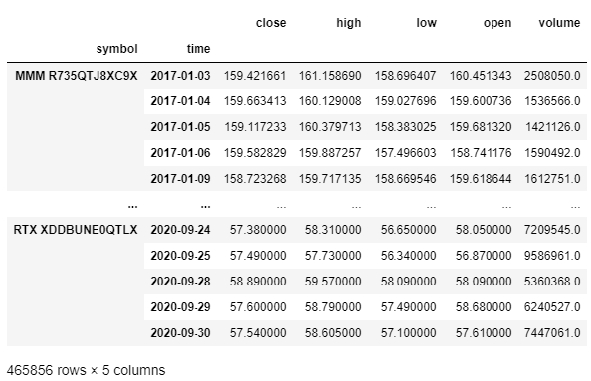
This is going to create a MultiIndex Dataframe with the historical OHLCV daily data needed for analysis.
factorAnalysis.ohlcvDf
Create Factors
Now we are going to create two very simple factors, Momentum and Volatility, using the CustomFactor function as follows.
# example of calculating multiple factors using the CustomFactor function

from scipy.stats import skew, kurtosis

def CustomFactor(x):

'''
Description:
Applies factor calculations to a SingleIndex DataFrame of historical data OHLCV by symbol
Args:
x: SingleIndex DataFrame of historical OHLCV data for each symbol
Returns:
The factor value for each day
'''

try:
# momentum factor --------------------------------------------------------------------------
closePricesTimeseries = x['close'].rolling(252) # create a 252 day rolling window of close prices
returns = x['close'].pct_change().dropna() # create a returns series
momentum = closePricesTimeseries.apply(lambda x: (x[-1] / x[-252]) - 1)

# volatility factor ------------------------------------------------------------------------
volatility = returns.rolling(252).apply(lambda x: np.nanstd(x, axis = 0))

# get a dataframe with all factors as columns --------------------------------------------
factors = pd.concat([momentum, volatility], axis = 1)

except BaseException as e:
factors = np.nan

return factors
What's going on there?
- Under the hood, this function gets applied to the OHLCV DataFrame grouped by symbol. That means we can perform calculations for each symbol using any of the OHLCV columns in the grouped 'x' DataFrame.
- We want to calculate factors in a rolling fashion so we get a value for each day that is calculated using data up until that day and including that day. By doing this we assume that in backtesting (and live trading) the calculations and trading decisions happen after the market closes and before the next open.
- Finally, we concatenate the factors so we get the resulting DataFrame with one column per factor.
# example of a multiple factors
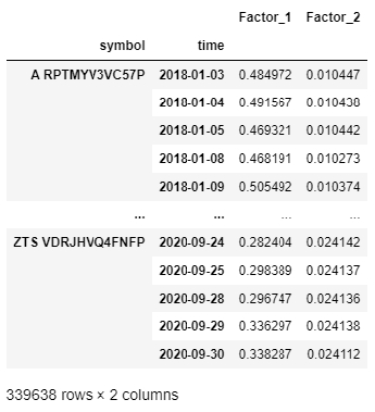
factorsDf = factorAnalysis.GetFactorsDf(CustomFactor)
factorsDf
In order to standardize the data, we apply winsorization and zscore normalization. We won't go over that here so please refer to the Notebook for more information on this.
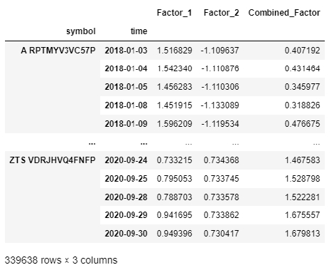
We have two single factors and we want to combine them into one factor that is some linear combination of the two. We do this using the combinedFactorWeightsDict that takes the factor names and the weights. Note how we could reverse the effect of a factor by assigning a negative weight here. In this example, we will just sum the two.
# dictionary containing the factor name and weights for each factor
combinedFactorWeightsDict = {'Factor_1': 1, 'Factor_2': 1}
#combinedFactorWeightsDict = None # None to not add a combined factor when using single factors

finalFactorsDf = factorAnalysis.GetCombinedFactorsDf(standardizedFactorsDf, combinedFactorWeightsDict)
finalFactorsDf
Create Quantiles And Add Forward Returns
It is time to create our factor quantiles and calculate forward returns in order to assess the relationship between the two.
# inputs for forward returns calculations
field = 'open' # choose between open, high, low, close prices to calculate returns
forwardPeriods = [1, 5, 21] # choose periods for forward return calculations
# inputs for quantile calculations
factor = 'Combined_Factor' # choose a factor to create quantiles
q = 5 # choose the number of quantile groups to create
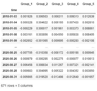
factorQuantilesForwardReturnsDf = factorAnalysis.GetFactorQuantilesForwardReturnsDf(finalFactorsDf, field,
forwardPeriods,
factor, q)
factorQuantilesForwardReturnsDf
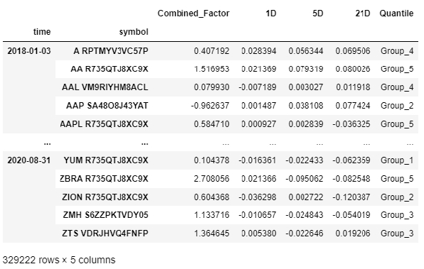
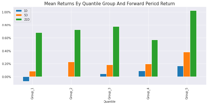
- In order to calculate forward returns, we need to choose the price we want to use for that and the different periods we want to get. In this example, we are calculating the 1, 5 and 21 forward returns based on Open prices. We use Open prices in order to replicate how the event-driven backtesting will work: we make all calculations after the market close (with data up until then and including that data point) and rebalance positions at the market open.
- We select the factor we want to use for the quantiles and how many quantile groups we want to create. We are using the Combined_Factor and 5 quintiles here.
Let's have a look at the mean returns.
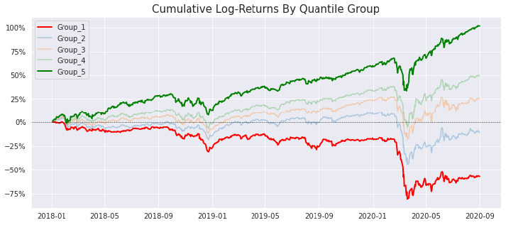
The next step is to visualize the cumulative returns from each quintile over time. In order to do that, we are going to group by quintile every day and calculate the return for each quintile/day by either using equal-weighting (mean) or factor-based weighting (weight the return of each stock in the quintile by its factor value).
forwardPeriod = 1 # choose the forward period to use for returns
weighting = 'mean' # mean/factor

returnsByQuantileDf = factorAnalysis.GetReturnsByQuantileDf(factorQuantilesForwardReturnsDf,
forwardPeriod, weighting)
returnsByQuantileDf
Here we are ideally looking for returns series that deviate from each other in the direction of the quintiles order (top quintile going up while bottom quintile going down).
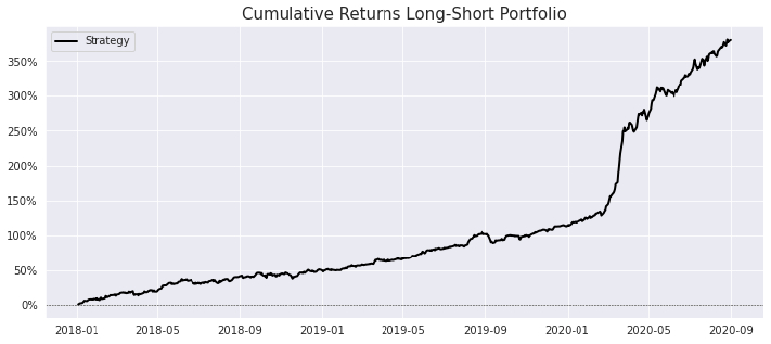
Create a Long-Short Portfolio
We are finally in a position to construct a portfolio that exploits the spread between the top and bottom quintiles. In order to do this, we need to select two quintiles and provide some weighting that we want to apply to each of them using the portfolioWeightsDict. This allows for some flexibility in the way we create the portfolio as we can give more or less weight to one of the quintiles.
# dictionary containing the quintile group names and portfolio weights for each
portfolioWeightsDict = {'Group_5': 1, 'Group_1': -1}

portfolioLongShortReturnsDf = factorAnalysis.GetPortfolioLongShortReturnsDf(returnsByQuantileDf, portfolioWeightsDict)
portfolioLongShortReturnsDf
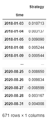
And the plot!
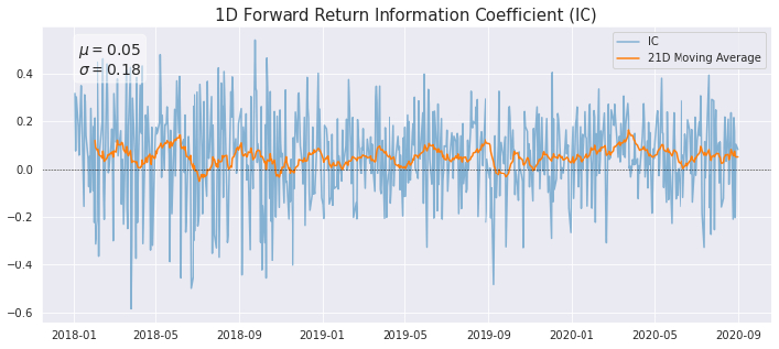
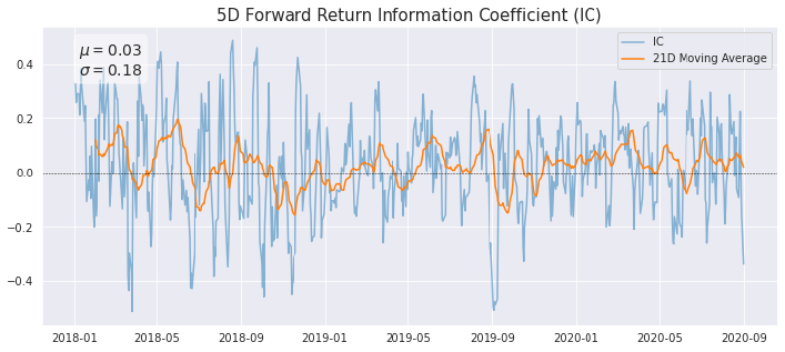
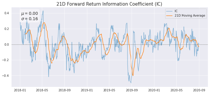
Spearman Rank Correlation Coefficient
A standard way of assessing the degree of correlation between our factor and forward returns is the Spearman Rank Correlation (Information Coefficient).
The Spearman Rank Correlation measures the strength and direction of association between two ranked variables. It is the non-parametric version of the Pearson correlation and focuses on the monotonic relationship between two variables rather than their linear relationship. Below we plot the daily IC between the factor values and each forward period return, along with a 21-day moving average.
factorAnalysis.PlotIC(factorQuantilesForwardReturnsDf)
CASE STUDY - RISK RESEARCH
This section corresponds to the RiskAnalysis class whose purpose is to discover what risk factors our strategy is exposed to and to what degree. As we will see below in more detail, these external factors can be any time series of returns that our portfolio could have some exposure to. Some popular risk factors are provided here (Fama-French Five Factors, Industry Factors), but the user can easily test any other by passing its time series of returns. The Notebook also contains detailed step by step instructions.
Initialize Data
Let's initialize the RiskAnalysis class.
# initialize risk analysis
riskAnalysis = RiskAnalysis(qb)
After initializing the RiskAnalysis class, we get two datasets with classic risk factors:
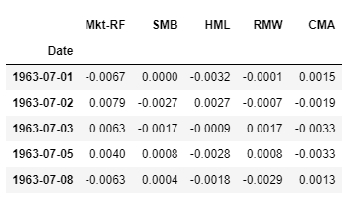
- Fama-French 5 Factors: Historical daily returns of Market Excess Return (Mkt-RF), Small Minus Big (SMB), High Minus Low (HML), Robust Minus Weak (RMW) and Conservative Minus Aggressive (CMA).
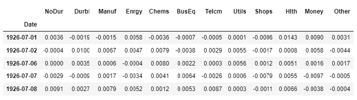
- 12 Industry Factors: Consumer Nondurables (NoDur), Consumer durables (Durbl), Manufacturing (Manuf), Energy (Enrgy), Chemicals (Chems), Business Equipment (BusEq), Telecommunications (Telcm), Utilities (Utils), Wholesale and Retail (Shops), Healthcare (Hlth), Finance (Money), Other (Other)
Visit this site for more factor datasets to add to this analysis.
# fama-french 5 factors
riskAnalysis.ffFiveFactorsDf.head()
# 12 industry factors
riskAnalysis.industryFactorsDf.head()
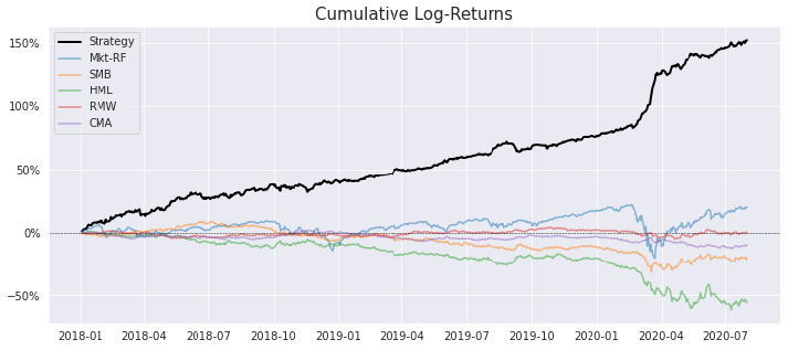
Let's take a look at the cumulative returns of our long-short strategy together with the returns of the Fama-French 5 Factors.
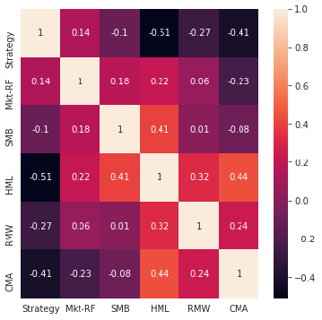
We can visualize the correlations between the risk factors and our strategy returns.
# plot correlation matrix
factorAnalysis.PlotFactorsCorrMatrix(combinedReturnsDf))
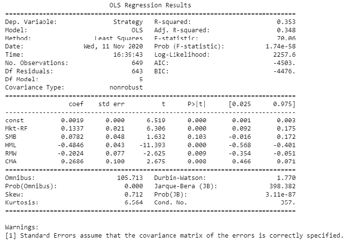
Run Regression Analysis
- Fit a Regression Model to the data to analyse linear relationships between our strategy returns and the external risk factors.
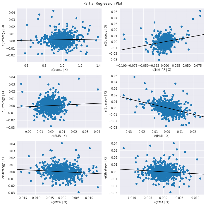
- Partial Regression plots. When performing multiple linear regression, these plots are useful in analysing the relationship between each independent variable and the response variable while accounting for the effect of all the other independent variables peresent in the model. Calculations are as follows (Wikipedia):
- Compute the residuals of regressing the response variable against the independent variables but omitting Xi.
- Compute the residuals from regressing Xi against the remaining independent variables.
- Plot the residuals from (1) against the residuals from (2).
riskAnalysis.PlotRegressionModel(combinedReturnsDf, dependentColumn = 'Strategy')
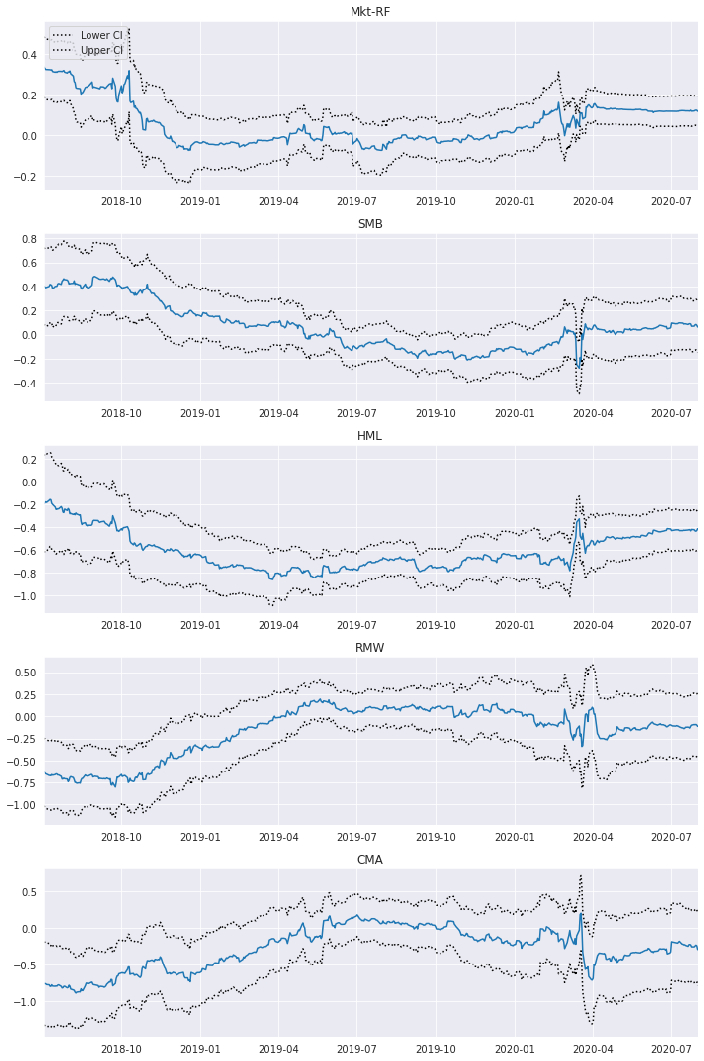
Plot Rolling Regression Coefficients
The above relationships are not static through time, therefore it is useful to visualize how these coefficients behave over time by running a Rolling Regression Model (with a given lookback period).
riskAnalysis.PlotRollingRegressionCoefficients(combinedReturnsDf, dependentColumn = 'Strategy', lookback = 126)
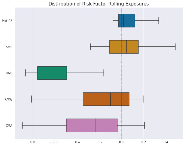
Plot Distribution Of Rolling Exposures
We can now visualize the historical distributions of the rolling regression coefficients in order to get a better idea of the variability of the data.
riskAnalysis.PlotBoxPlotRollingFactorExposure(combinedReturnsDf, dependentColumn = 'Strategy', lookback = 126)
CASE STUDY - BACKTESTING ALGORITHM
The purpose of the research process illustrated above is purely to determine if there is a significant relationship between our factors and the future returns of those stocks. That means the cumulative returns we saw are not realistic and they assumed daily rebalancing of hundreds of stocks without accounting for any slippage or commissions.
In order to test how this strategy would have performed historically we need to run a proper backtest, and for that we have to move from the Research Notebook to the Algorithm Framework.
Below I will explain the most important features and scripts of this part of the product.
Algorithm Framework - main.py
The main.py script includes the follwing user-defined inputs worth mentioning.
# date rule for rebalancing our portfolio by updating long-short positions based on factor values
rebalancingFunc = Expiry.EndOfMonth

# number of stocks to keep for factor modelling calculations
nStocks = 100

# number of positions to hold on each side (long/short)
positionsOnEachSide = 20

# lookback for historical data to calculate factors
lookback = 252

# select the leverage factor
leverageFactor = 1
- We first need to select how often we want to rebalance the portfolio (i.e. recalculate all factors and portfolio weights). Here you can choose among a number of date rules such as
Expiry.EndOfMonth - At every rebalancing, the algorithm will create a dynamic universe of stocks based on DollarVolume and MarketCap that will be used to calculate the factors on (
nStocks) and ultimately select the top and bottom stocks to trade (positionsOnEachSide). - Finally, we need to decide how much historical data we want for our factors calculations using
lookback - There is also a
leverageFactorparameter that can be used to modify the account leverage.
Algorithm Framework - classSymbolData.py
The Backtesting Algorithm has been designed to make it easy to quickly add and remove the factors previously analysed in the notebook. We only need to add the function that calculates the factor to the SymbolData class. For example, have a look at how we add the Momentum and Volatility factors from before.
def CalculateMomentum(self, history):

closePrices = history.loc[self.Symbol]['close']
momentum = (closePrices[-1] / closePrices[-252]) - 1

return momentum

def CalculateVolatility(self, history):

closePrices = history.loc[self.Symbol]['close']
returns = closePrices.pct_change().dropna()
volatility = np.nanstd(returns, axis = 0)

return volatility
You can add as many functions as you want and then simply include them or exclude them from the strategy by simply commenting out the function call here. Note how there are a few functions for other factors that we commented out to leave out of the strategy.
def CalculateFactors(self, history, fundamentalDataBySymbolDict):

self.fundamentalDataDict = fundamentalDataBySymbolDict[self.Symbol]
self.momentum = self.CalculateMomentum(history)
self.volatility = self.CalculateVolatility(history)
#self.skewness = self.CalculateSkewness(history)
#self.kurt = self.CalculateKurtosis(history)
#self.distanceVsHL = self.CalculateDistanceVsHL(history)
#self.meanOvernightReturns = self.CalculateMeanOvernightReturns(history)
And at the end we just need to add the chosen factors to the property factorsList
@propertyAlgorithm Framework - HelperFunctions.py
def factorsList(self):
technicalFactors = [self.momentum, self.volatility]
In the Research Notebook we could only add factors created using OHLCV data for the reasons already stated above. However, the Backtesting Algorithm allows to add fundamental factors very easily by using the GetFundamentalDataDict function. As you can see below, we create a dictionary containing the fundamental ratio and its desired direction in the model (1 for a positive effect or -1 for a negative one). For a list of all the fundamental data available in QuantConnect please refer to this page https://www.quantconnect.com/docs/data-library/fundamentals
# dictionary of symbols containing factors and the direction of the factor (1 for sorting descending and -1 for sorting ascending)
fundamentalDataBySymbolDict[x.Symbol] = {
#fundamental.ValuationRatios.BookValuePerShare: 1,
#fundamental.FinancialStatements.BalanceSheet.TotalEquity.Value: -1,
#fundamental.OperationRatios.OperationMargin.Value: 1,
#fundamental.OperationRatios.ROE.Value: 1,
#fundamental.OperationRatios.TotalAssetsGrowth.Value: 1,
#fundamental.ValuationRatios.PERatio: 1}
Finally, very much like we did in the Research Notebook, in the Backtesting Algorithm we can also give different weights to each factor to create a combined factor. We do that using the GetLongShortLists function in the HelperFunctions.py script as per below.
normFactorsDf['combinedFactor'] = normFactorsDf['Factor_1'] * 1 + normFactorsDf['Factor_2'] * 1CLONE THE ALGORITHM
And that was it! Now you can clone the below algorithm into your QuantConnect account and start playing with the different features yourself. The algorithm also has a number of interesting backtesting charts such as Drawdown and Total Portfolio Exposure %, so remember to activate those on the Select Chart box (top right corner of backtesting page).
-------------
Thank you!
Emilio
======================
20210330 - NOTE: This was updated in the comment below to deal with a look ahead bias:
https://www.quantconnect.com/forum/discussion/9768/factor-investing-in-quantconnect-research-notebook-amp-backtesting-algorithm/p1/comment-31435


Spacetime
amazing! thank you!
Sebastian Brocklesby
This is great. Thank you.
Rémy Heinis
That's really great work thank you !
Laurent Crouzet
Thanks a lot, Emilio! The QC community will most probably profit from the sharing of such a good research!
Ben Zhang
Hello Emilio,
Awesome work with the factor-based modeling! I was wondering if there was a way to include the stocks in the SP500 on a rolling basis. I noticed that the constituents are current and don't take into account delistings! Is there a way to include on a rolling basis the stocks that are part of the index?
Also awesome work with the risk decompositions! I really enjoyed playing around with the notebook!
Emilio Freire
Thank you all for the kind comments!
Ben Zhang Unfortunately QuantConnect does not support dynamic universe selection in the Research Notebook as of now, only in the backtesting engine. I believe it's a feature in their pipeline though. In order to build this notebook I had to provide a static list of current SP500 tickers for now, but hopefully in the near future we will be able to create universes like the rolling SP500 index in the Research Notebook and this product will become more powerful!
Thanks,
Emilio
Vladimir
Emilio Freire
A very detailed study deserves a special reward.
I have back tested the strategy from 2007, 6, 1.
It works, like most long-short strategies, only at the beginning of bear markets.
I think Long - Bond strategy will perform much better.
Try that.
Emilio Freire
Thanks Vladimir !
I will test it out.
Emilio
Vladimir
Emilio Freire
It will be good to have this simple Stock-Bond Portfolio as a bankmark to surpass.
Vladimir
Emiliano Fraticelli
Thank you so much @emilio
Erol Aspromatis
This is amazing work Emilio and I will be spending my Holiday going through this model. I'm particullarly interestead in leveraging this for factor investing.
Your strategy here has done such an amazing job ourperforming the other traditional five FF factors, particullarly the HML (value factor) in the backtest. The momentum factor has obviously been huge in hindsight, but my hypothis is that we will eventually see some type of mean reversion, which could indicate that the value factor will perhaps to better in the future.
Anyway, this gives me a great framework to start testing and developing.
Emilio Freire
Thank you Erol Aspromatis !
Great to see this project is helping the community.
Please do not hesitate to ask questions here if needed about the code and overall algo. I will try my best to answer them :)
Enjoy your holidays!
Emilio
ASHOK MEHTA
Hi Emilio, This very good description of using a research notebook. I am very new to Quant Connect, hence don't yet know how can I see the code in your notebook. Looks like there is a link to clone the algorithm, but nothing to clone the notebook. If you don't mind can you please share the notebook. Thanks
Ashok
Emilio Freire
Hi ASHOK MEHTA !
The research notebook is part of the algorithm as you can see in the below screenshot. When you click on Clone Algorithm you will get a copy of the whole project in your QuantConnect account. To open the notebook simply open the research.ipynb file!
Fabmei
Hello Emilio,
this is great for learning and the detailed desciption helps a lot creating and working with dataframes. Thank you! One question regarding the universe selection: I can't seem to figure out where the tickers are added - maybe missing the forest for the trees there. An answer would help a lot working with the algo and trying out different universes. Could you please give some description on that as well?
Best, Fabmei
Emiliano Fraticelli
Hi!
In order to say test factors based on fundamentals like , for instance, Free Cash Flow Yield, using this notebook? It seems you get the CustomFactor by usig close price and later volatility, all things that could be build from the OHLCV df. I'm worried that in order to test factors like the one I mentioned on FCF I should build a strategy on QC, export the return series via .json, uploading it to dropbox, and then finally import the return series on the notebook.
Am I wrong?
Thanks
Derek Melchin
Hi Fabmei,
The tickers are subscribed to through a custom coarse-fine universe selection model. In the Initialize method in main.py, we see
self.SetUniverseSelection(FactorModelUniverseSelectionModel(benchmark = benchmark,
                                                            nStocks = nStocks,
                                                            lookback = lookback,
                                                            maxNumberOfPositions = maxNumberOfPositions,
                                                            rebalancingFunc = rebalancingFunc))
Refer to our documentation on Universe Selection for more information.
Hi Emiliano,
When switching the factor used in the notebook above, we don't need to run a backtest. The `GetFactorsDf` method in the notebook above returns a DataFrame with the technical factor values at each timestep. The notebook below demonstrates how we can get the FCF fundamental factor into a similar timeseries DataFrame. To merge this fundamental factor logic into the factor analysis notebook above, we just need to define a method like `GetFactorsDf` that uses fundamental factors.
Best,
Derek Melchin
The material on this website is provided for informational purposes only and does not constitute an offer to sell, a solicitation to buy, or a recommendation or endorsement for any security or strategy, nor does it constitute an offer to provide investment advisory services by QuantConnect. In addition, the material offers no opinion with respect to the suitability of any security or specific investment. QuantConnect makes no guarantees as to the accuracy or completeness of the views expressed in the website. The views are subject to change, and may have become unreliable for various reasons, including changes in market conditions or economic circumstances. All investments involve risk, including loss of principal. You should consult with an investment professional before making any investment decisions.
EpsilonOcean
Excellent post. There's a future leak in the presented factor (I had to figure out why performance was so spectacular).
If you're using close prices to create the factor, using open to evaluate it and shifting open prices backwards creates a future leak.
Thanks for the framework, will use it.
Emilio Freire
Hi EpsilonOcean !
Thanks a lot for that. You're right. There's a half-day look ahead! I was trying to replicate the behaviour of the backtest but I guess the only way is to use close prices to evaluate the factor and that's it? In a backtest we wouldn't get the close to close return but rather open to close return so I was trying to achieve that and introduced the look ahead in the process.
You fixed it by just using 'close' instead of 'open', right? Can you think of any other way to get closer to backtest behaviour?
Thanks!
Emilio
EpsilonOcean
Hey, yep I just used Close not Open... So I guess we would just have to be mindful of what data is going in and coming out when using the factor scripts.
I dont think you necessarily need to match backtest perfectly when looking at a factor in research, it's just a really great way to see if there is a predictive component in an idea - then we can combine/alter etc as we wish before the backtest. Quantile spreads are handly too - as a check that it will beat costs.
There have been a papers recently replicating academic factor studies I'm keen to check out with your framework!
Emilio Freire
The material on this website is provided for informational purposes only and does not constitute an offer to sell, a solicitation to buy, or a recommendation or endorsement for any security or strategy, nor does it constitute an offer to provide investment advisory services by QuantConnect. In addition, the material offers no opinion with respect to the suitability of any security or specific investment. QuantConnect makes no guarantees as to the accuracy or completeness of the views expressed in the website. The views are subject to change, and may have become unreliable for various reasons, including changes in market conditions or economic circumstances. All investments involve risk, including loss of principal. You should consult with an investment professional before making any investment decisions.
To unlock posting to the community forums please complete at least 30% of Boot Camp.
You can continue your Boot Camp training progress from the terminal. We hope to see you in the community soon!