Combined Carry and Trend

Introduction

In this research, we build upon the Futures Fast Trend Following strategy to widen the universe of Futures and increase the number of factors we consider when forming a portfolio. In the previous strategy, we used a single exponential moving average crossover (EMAC) trend filter to forecast future returns. In this iteration of the strategy, we incorporate several EMAC trend forecasts and several carry forecasts. Trending strategies are a divergent style of strategy whereas carry strategies are a convergent style of strategy. The results show that by using both styles of strategies in one algorithm, we can diversify our factor exposures and improve the risk-adjusted returns. This algorithm is a re-creation of strategy #11 from Advanced Futures Trading Strategies (Carver, 2023), but Carver doesn’t endorse and hasn’t reviewed this implementation. 

Background

The adjusted price of a Future (the continuous contract price) doesn’t exactly match the underlying spot price because the adjusted price includes returns from changes in the underlying spot price and returns from carry.

\[\textrm{Excess return} = \textrm{Spot return} + \textrm{Carry}\]

The adjusted price is simply the cumulative excess return in the preceding formula. The source of the carry return depends on the asset class of the instrument you’re trading. You can find the source of carry by thinking about an arbitrage trade that would replicate a long position in the Future. For example, to replicate a position in an S&P 500 Index Future, you would borrow money to buy all of the stocks in the Index and you would receive dividends as a benefit. Therefore, the carry would be the expected dividends you would receive before the Future expires minus the interest rate you would pay to borrow the money.

\[\textrm{Carry (Equities)} = \textrm{Dividends} - \textrm{Interest}\]

For example, in Forex, carry is the deposit rate minus the borrowing rate. For agricultural goods, carry is the convenience yield minus the sum of borrowing and storage costs.

However, there is an alternative method for calculating carry, which involves comparing the prices between two consecutive contracts. For example, say you’re trading a Future that has monthly contracts. The contract expiring today is priced at $100, the contract expiring after that is priced at $99, and the following contract is priced at $98. If you buy the $99 contract and the underlying spot price doesn’t change, you can expect the contract to be worth $100 at expiry, earning you a carry of $1.

Positive carry exists because if you buy a Future with positive expected carry, you are essentially being rewarded for providing insurance against price depreciation in the underlying asset.

Carry Forecasts

We can use the expected carry of a Future to produce forecasts in a trading strategy. As mentioned above, the expected carry is the price difference between two consecutive Futures contracts. For a mathematical explanation of how Carver forecasts carry, see chapter 11 of Advanced Futures Trading Strategies.

Trend Forecasts

The Fast Trend Following strategy used a single EMAC(16, 64) trend filter to produce forecasts. In this strategy, use the following filters:

• EMAC(16, 64)
• EMAC(32, 128)
• EMAC(64, 256)

The process of calculating the trend forecast is similar to the Fast Trend Following strategy, except we change the forecast scalar based on the EMAC span.

\[\textrm{Raw forecast} = \frac{EMAC(n,4n)}{\sigma_{\%,t}}\]

\[\textrm{Scaled forecast} = \textrm{Raw forecast} \times \textrm{Forecast scalar}\]

\[\textrm{Capped forecast} = \max(\min(\textrm{Scaled forecast}, 20), -20)\]

Aggregating Forecasts

This strategy has two components, a divergent-style EMAC trend forecast and a convergent-style smoothed carry forecast. Moreover, each component has several variations. For example, we have EMAC(16, 64), EMAC(64, 256), Carry(5), and Carry(20). What weighting scheme should we use to aggregate all these forecasts? Carver found that a 40% weight for the convergent style, a 60% weight for the divergent style, and an equal weight for each variation in each style produces the greatest Sharpe ratio. After aggregating the forecasts of each style using the 60%-40% mix, we apply a forecast diversification multiplier to keep the average forecast at a value of 10 and then cap the result to be within the interval [-20, 20].

Method

Let’s walk through how we can implement this trading algorithm with the LEAN trading engine.

Initialization

We start with the Initialization method, where we set the start date, end date, cash, and some settings.

class FuturesCombinedCarryAndTrendAlgorithm(QCAlgorithm):
    
    def Initialize(self):
        self.SetStartDate(2020, 7, 1)
        self.SetEndDate(2023, 7, 1)
        self.SetCash(1_000_000)

        self.SetBrokerageModel(BrokerageName.InteractiveBrokersBrokerage, AccountType.Margin)
        self.SetSecurityInitializer(BrokerageModelSecurityInitializer(self.BrokerageModel, FuncSecuritySeeder(self.GetLastKnownPrices)))        
        self.Settings.MinimumOrderMarginPortfolioPercentage = 0

Universe Selection

We increase the universe size from the Fast Trend Following strategy to include 10 different Futures. To accomplish this, follow these steps:

1. In the futures.py file, create some FutureData objects, which hold the Future Symbol, market category, and the contract offset. 

The contract offset represents which contract in the chain to trade. 0 represents the front-month contract, 1 represents the contract that expires next, and so on. In this example, we follow Carver and trade the second contract in the chain for natural gas Futures to reduce the seasonality effect.

class FutureData:
    def __init__(self, classification, contract_offset):
        self.classification = classification
        self.contract_offset = contract_offset

categories = {
    pair[0]: FutureData(pair[1], pair[2]) for pair in [
        (Symbol.Create(Futures.Indices.SP500EMini, SecurityType.Future, Market.CME), ("Equity", "US"), 0),
        (Symbol.Create(Futures.Indices.NASDAQ100EMini, SecurityType.Future, Market.CME), ("Equity", "US"), 0),
        (Symbol.Create(Futures.Indices.Russell2000EMini, SecurityType.Future, Market.CME), ("Equity", "US"), 0),
        (Symbol.Create(Futures.Indices.VIX, SecurityType.Future, Market.CFE), ("Volatility", "US"), 0),
        (Symbol.Create(Futures.Energies.NaturalGas, SecurityType.Future, Market.NYMEX), ("Energies", "Gas"), 1),
        (Symbol.Create(Futures.Energies.CrudeOilWTI, SecurityType.Future, Market.NYMEX), ("Energies", "Oil"), 0),
        (Symbol.Create(Futures.Grains.Corn, SecurityType.Future, Market.CBOT), ("Agricultural", "Grain"), 0),
        (Symbol.Create(Futures.Metals.Copper, SecurityType.Future, Market.COMEX), ("Metals", "Industrial"), 0),
        (Symbol.Create(Futures.Metals.Gold, SecurityType.Future, Market.COMEX), ("Metals", "Precious"), 0),
        (Symbol.Create(Futures.Metals.Silver, SecurityType.Future, Market.COMEX), ("Metals", "Precious"), 0)
    ]
}

2. In the universe.py file, import the categories and define the Universe Selection model.

from Selection.FutureUniverseSelectionModel import FutureUniverseSelectionModel
from futures import categories

class AdvancedFuturesUniverseSelectionModel(FutureUniverseSelectionModel):
    def __init__(self) -> None:
        super().__init__(timedelta(1), self.select_future_chain_symbols)
        self.symbols = list(categories.keys())

    def select_future_chain_symbols(self, utc_time: datetime) -> List[Symbol]:
        return self.symbols

    def Filter(self, filter: FutureFilterUniverse) -> FutureFilterUniverse:
        return filter.Expiration(0, 365)

3. In the main.py file, extend the Initialization method to configure the universe settings and add the Universe Selection model. 

class FuturesCombinedCarryAndTrendAlgorithm(QCAlgorithm):
    def Initialize(self):
        # . . .
        self.UniverseSettings.DataNormalizationMode = DataNormalizationMode.BackwardsPanamaCanal
        self.UniverseSettings.DataMappingMode = DataMappingMode.LastTradingDay
        self.AddUniverseSelection(AdvancedFuturesUniverseSelectionModel())

Note that the original algorithm by Carver rolls over contracts \(n\) days before they expire instead on the last day, so our results will be slightly different.

Forecasting Carry and Trend

We first define the constructor of the Alpha model in the alpha.py file.

class CarryAndTrendAlphaModel(AlphaModel):

    futures = []
    BUSINESS_DAYS_IN_YEAR = 256
    TREND_FORECAST_SCALAR_BY_SPAN = {64: 1.91, 32: 2.79, 16: 4.1, 8: 5.95, 4: 8.53, 2: 12.1} # Table 29 on page 177
    CARRY_FORECAST_SCALAR = 30 # Provided on p.216
    FDM_BY_RULE_COUNT = { # Table 52 on page 234
        1: 1.0,
        2: 1.02,
        3: 1.03,
        4: 1.23,
        5: 1.25,
        6: 1.27,
        7: 1.29,
        8: 1.32,
        9: 1.34,
    }

    def __init__(self, algorithm, emac_filters, abs_forecast_cap, sigma_span, target_risk, blend_years):
        self.algorithm = algorithm
        
        self.emac_spans = [2**x for x in range(4, emac_filters+1)]
        self.fast_ema_spans = self.emac_spans
        self.slow_ema_spans = [fast_span * 4 for fast_span in self.emac_spans]
        self.all_ema_spans = sorted(list(set(self.fast_ema_spans + self.slow_ema_spans)))

        self.carry_spans = [5, 20, 60, 120]

        self.annulaization_factor = self.BUSINESS_DAYS_IN_YEAR ** 0.5

        self.abs_forecast_cap = abs_forecast_cap
        
        self.sigma_span = sigma_span
        self.target_risk = target_risk
        self.blend_years = blend_years

        self.idm = 1.5  # Instrument Diversification Multiplier. 

        self.categories = categories
        self.total_lookback = timedelta(sigma_span*(7/5) + blend_years*365)

        self.day = -1

When new Futures are added to the universe, we gather some historical data and set up a consolidator to keep the trailing data updated as the algorithm executes. If the security that’s added is a continuous contract, we combine two EMA indicators to create the EMAC.

class CarryAndTrendAlphaModel(AlphaModel):

    def OnSecuritiesChanged(self, algorithm: QCAlgorithm, changes: SecurityChanges) -> None:
        for security in changes.AddedSecurities:
            symbol = security.Symbol

            # Create a consolidator to update the history
            security.consolidator = TradeBarConsolidator(timedelta(1))
            security.consolidator.DataConsolidated += self.consolidation_handler
            algorithm.SubscriptionManager.AddConsolidator(symbol, security.consolidator)

            # Get raw and adjusted history
            security.raw_history = pd.Series()

            if symbol.IsCanonical():
                security.adjusted_history = pd.Series()
                security.annualized_raw_carry_history = pd.Series()

                # Create indicators for the continuous contract
                ema_by_span = {span: algorithm.EMA(symbol, span, Resolution.Daily) for span in self.all_ema_spans}
                security.ewmac_by_span = {}
                for i, fast_span in enumerate(self.emac_spans):
                    security.ewmac_by_span[fast_span] = IndicatorExtensions.Minus(ema_by_span[fast_span], ema_by_span[self.slow_ema_spans[i]])

                security.automatic_indicators = ema_by_span.values()

                self.futures.append(security)

        for security in changes.RemovedSecurities:
            # Remove consolidator + indicators
            algorithm.SubscriptionManager.RemoveConsolidator(security.Symbol, security.consolidator)
            if security.Symbol.IsCanonical():
                for indicator in security.automatic_indicators:
                    algorithm.DeregisterIndicator(indicator)

The consolidation handler simply updates the security history and trims off any history that’s too old.

class CarryAndTrendAlphaModel(AlphaModel):
    def consolidation_handler(self, sender: object, consolidated_bar: TradeBar) -> None:
        security = self.algorithm.Securities[consolidated_bar.Symbol]
        end_date = consolidated_bar.EndTime.date()
        if security.Symbol.IsCanonical():
            # Update adjusted history
            security.adjusted_history.loc[end_date] = consolidated_bar.Close
            security.adjusted_history = security.adjusted_history[security.adjusted_history.index >= end_date - self.total_lookback]
        else:
            # Update raw history
            continuous_contract = self.algorithm.Securities[security.Symbol.Canonical]
            if hasattr(continuous_contract, "latest_mapped") and consolidated_bar.Symbol == continuous_contract.latest_mapped:
                continuous_contract.raw_history.loc[end_date] = consolidated_bar.Close
                continuous_contract.raw_history = continuous_contract.raw_history[continuous_contract.raw_history.index >= end_date - self.total_lookback]
            
            # Update raw carry history
            security.raw_history.loc[end_date] = consolidated_bar.Close
            security.raw_history = security.raw_history.iloc[-1:]

The Update method calculates the forecast of the Futures at the beginning of each trading day and returns some Insight objects for the Portfolio Construction model.

class CarryAndTrendAlphaModel(AlphaModel):
    def Update(self, algorithm: QCAlgorithm, data: Slice) -> List[Insight]:
        if data.QuoteBars.Count:
            for future in self.futures:
                future.latest_mapped = future.Mapped

        # Rebalance daily
        if self.day == data.Time.day or data.QuoteBars.Count == 0:
            return []

        # Update annualized carry data
        for future in self.futures:
            # Get the near and far contracts
            contracts = self.get_near_and_further_contracts(algorithm.Securities, future.Mapped)
            if contracts is None:
                continue
            near_contract, further_contract = contracts[0], contracts[1]
            
            # Save near and further contract for later
            future.near_contract = near_contract
            future.further_contract = further_contract

            # Check if the daily consolidator has provided a bar for these contracts yet
            if not hasattr(near_contract, "raw_history") or not hasattr(further_contract, "raw_history") or near_contract.raw_history.empty or further_contract.raw_history.empty:
                continue
            # Update annualized raw carry history
            raw_carry = near_contract.raw_history.iloc[0] - further_contract.raw_history.iloc[0]
            months_between_contracts = round((further_contract.Expiry - near_contract.Expiry).days / 30)
            expiry_difference_in_years = abs(months_between_contracts) / 12
            annualized_raw_carry = raw_carry / expiry_difference_in_years
            future.annualized_raw_carry_history.loc[near_contract.raw_history.index[0]] = annualized_raw_carry

        # If warming up and still > 7 days before start date, don't do anything
        # We use a 7-day buffer so that the algorithm has active insights when warm-up ends
        if algorithm.StartDate - algorithm.Time > timedelta(7):
            self.day = data.Time.day
            return []
        
        # Estimate the standard deviation of % daily returns for each future
        sigma_pcts_by_future = {}
        for future in self.futures:
            sigma_pcts = self.estimate_std_of_pct_returns(future.raw_history, future.adjusted_history)
            # Check if there is sufficient history
            if sigma_pcts is None:
                continue
            sigma_pcts_by_future[future] = sigma_pcts

        # Create insights
        insights = []
        weight_by_symbol = GetPositionSize({future.Symbol: self.categories[future.Symbol].classification for future in sigma_pcts_by_future.keys()})
        for symbol, instrument_weight in weight_by_symbol.items():
            future = algorithm.Securities[symbol]
            target_contract = [future.near_contract, future.further_contract][self.categories[future.Symbol].contract_offset]
            sigma_pct = sigma_pcts_by_future[future]
            daily_risk_price_terms = sigma_pct / (self.annulaization_factor) * target_contract.Price # "The price should be for the expiry date we currently hold (not the back-adjusted price)" (p.55)

            # Calculate target position
            position = (algorithm.Portfolio.TotalPortfolioValue * self.idm * instrument_weight * self.target_risk) \
                        /(future.SymbolProperties.ContractMultiplier * daily_risk_price_terms * (self.annulaization_factor))

            # Calculate forecast type 1: EMAC
            trend_forecasts = self.calculate_emac_forecasts(future.ewmac_by_span, daily_risk_price_terms)
            if not trend_forecasts:
                continue
            emac_combined_forecasts = sum(trend_forecasts) / len(trend_forecasts) # Aggregate EMAC factors -- equal-weight

            # Calculate factor type 2: Carry
            carry_forecasts = self.calculate_carry_forecasts(future.annualized_raw_carry_history, daily_risk_price_terms)
            if not carry_forecasts:
                continue
            carry_combined_forecasts = sum(carry_forecasts) / len(carry_forecasts) # Aggregate Carry factors -- equal-weight
            
            # Aggregate factors -- 60% for trend, 40% for carry
            raw_combined_forecast = 0.6 * emac_combined_forecasts + 0.4 * carry_combined_forecasts
            scaled_combined_forecast = raw_combined_forecast * self.FDM_BY_RULE_COUNT[len(trend_forecasts) + len(carry_forecasts)] # Apply a forecast diversification multiplier to keep the average forecast at 10 (p 193-194)
            capped_combined_forecast = max(min(scaled_combined_forecast, self.abs_forecast_cap), -self.abs_forecast_cap)

            if capped_combined_forecast * position == 0:
                continue
            target_contract.forecast = capped_combined_forecast
            target_contract.position = position
            
            local_time = Extensions.ConvertTo(algorithm.Time, algorithm.TimeZone, future.Exchange.TimeZone)
            expiry = future.Exchange.Hours.GetNextMarketOpen(local_time, False) - timedelta(seconds=1)
            insights.append(Insight.Price(target_contract.Symbol, expiry, InsightDirection.Up if capped_combined_forecast * position > 0 else InsightDirection.Down))
        
        if insights:
            self.day = data.Time.day

        return insights

The calculate_emac_forecasts method calculates the EMAC forecasts.

class CarryAndTrendAlphaModel(AlphaModel):
    def calculate_emac_forecasts(self, ewmac_by_span, daily_risk_price_terms):
        forecasts = []
        for span in self.emac_spans:
            risk_adjusted_ewmac = ewmac_by_span[span].Current.Value / daily_risk_price_terms
            scaled_forecast_for_ewmac = risk_adjusted_ewmac * self.TREND_FORECAST_SCALAR_BY_SPAN[span]
            capped_forecast_for_ewmac = max(min(scaled_forecast_for_ewmac, self.abs_forecast_cap), -self.abs_forecast_cap)
            forecasts.append(capped_forecast_for_ewmac)
        return forecasts

The calculate_carry_forecasts method calculates the carry forecasts.

class CarryAndTrendAlphaModel(AlphaModel):
    def calculate_carry_forecasts(self, annualized_raw_carry, daily_risk_price_terms):
        carry_forecast = annualized_raw_carry / daily_risk_price_terms

        forecasts = []
        for span in self.carry_spans:
            ## Smooth out carry forecast
            smoothed_carry_forecast = carry_forecast.ewm(span=span, min_periods=span).mean().dropna()
            if smoothed_carry_forecast.empty:
                continue
            smoothed_carry_forecast = smoothed_carry_forecast.iloc[-1]
            ## Apply forecast scalar (p. 264)
            scaled_carry_forecast = smoothed_carry_forecast * self.CARRY_FORECAST_SCALAR
            ## Cap forecast
            capped_carry_forecast = max(min(scaled_carry_forecast, self.abs_forecast_cap), -self.abs_forecast_cap)
            forecasts.append(capped_carry_forecast)

        return forecasts

Finally, to add the Alpha model to the algorithm, we extend the Initialization method in the main.py file to set the new Alpha model.

from alpha import CarryAndTrendAlphaModel

class FuturesCombinedCarryAndTrendAlgorithm(QCAlgorithm):    
    def Initialize(self):
        # . . .
        self.AddAlpha(CarryAndTrendAlphaModel(
            self,
            self.GetParameter("emac_filters", 6), 
            self.GetParameter("abs_forecast_cap", 20),    # Hardcoded on p.173
            self.GetParameter("sigma_span", 32),          # Hardcoded to 32 on p.604
            self.GetParameter("target_risk", 0.2),        # Recommend value is 0.2 on p.75
            self.GetParameter("blend_years", 3)           # Number of years to use when blending sigma estimates
        ))

Calculating Position Sizes

This algorithm uses the same trade buffering logic as the Fast Trend Following strategy.

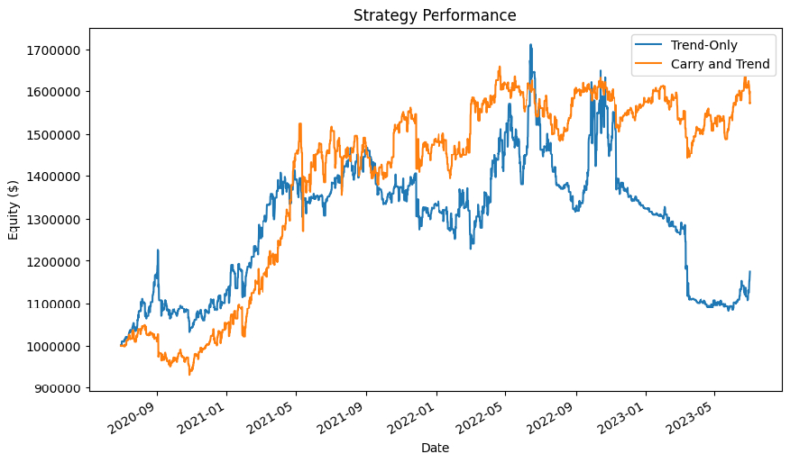
Results

We backtested the strategy from July 1, 2020 to July 1, 2023. The algorithm achieved a 0.749 Sharpe ratio. In contrast, the Fast Trend Following strategy, which only trades the trend component and uses a smaller universe, achieved a 0.294 Sharpe ratio over the same time period. Therefore, trading both carry and trend forecasts in a single algorithm increased the risk-adjusted returns of the portfolio. The following chart shows the equity curve of both strategies:

For more information about this strategy, see Advanced Futures Trading Strategies (Carver, 2023).

Further Research

If you want to continue developing this strategy, some areas of further research include:

• Adjusting parameter values
• Adding more uncorrelated varieties of the carry and trend forecasts
• Incorporating other factors besides carry and trend
• Adjusting the rollover timing to match the timing outlined by Carver
• Removing variations of the trend and carry forecast that are too expensive to trade after accounting for fees, slippage, and market impact

References

1. Carver, R. (2023). Advanced Futures Trading Strategies: 30 fully tested strategies for multiple trading styles and time frames. Harriman House Ltd.