


Hey everyone,In this post, I'm going to do my best to concisely explain what LSTM neural networks are and give an example of how to use them in your algorithm. If you want more information on LSTM, I highly recommend reading this post on how LSTM operates.
Recurrent neural networks (RNN) are an extremely powerful tool in deep learning. These models quite accurately mimic how humans process information and learn. Unlike traditional feedforward neural networks, RNNs have memory. That is, information fed into them persists and the network is able to draw on this to make inferences. In traditional neural networks, data is fed into the network and an output is produced. However, RNNs feed some information back into itself -- it decides to remember certain things rather than scraping all previous data. This functionality is massively powerful and has led to amazing achievements, but there is also a serious problem that accompanies RNNs -- the vanishing gradient.The vanishing gradient problem is essentially the inability of RNNs to handle long-term data dependencies. In neutral networks, gradients are found using backpropagation, which computes the gradient of the loss function with respect to the weights of the network. In backpropagation, the derivatives of each layer are multiplied down the network (from the final layer to the initial) to compute the derivatives of the initial layers. As more layers are added to the network, the chain-rule for derivatives means that small derivatives can compound quickly and the gradients of the loss function can approach zero. Such small gradients mean that the input weights for the initial layers can be so small that data is no longer recognized, effectively preventing the network from continuing to train.The solution to this problem is long short-term memory (LSTM), a type of recurrent neural network. Instead of one layer, LSTM cells generally have four, three of which are part of "gates" -- ways to optionally let information through. The three gates are commonly referred to as the forget, input, and output gates. The forget gate layer is where the model decides what information to keep from prior states. At the input gate layer, the model decides which values to update. Finally, the output gate layer is where the final output of the cell state is decided. Essentially, LSTM separately decides what to remember and the rate at which it should update. There is a lot of work that goes on behind the scenes here and this is just the broad strokes of what happens, but the essential difference between LSTM and n naive RNN is that LSTM is better equipped at handling long-term memory and avoids the vanishing gradient problem.
LSTM has been applied to fields as diverse as speech recognition, text recognition and translation, image processing, and robotic control. In addition to these fields, LSTM models have produced some great results when applied to time-series prediction. One of the central challenges with conventional time-series models is that, despite trying to account for trends or other non-stationary elements, it is almost impossible to truly predict an outlier like a recession, flash crash, liquidity crisis, etc. By having a long memory, LSTM models are better able to capture these difficult trends in the data without suffering from the level of overfitting a conventional model would need in order to capture the same data.
For a very basic application, we're going to use an LSTM model to predict the price movement, a non-stationary time-series, of SPY (the structure of the model setup below was adapted from this post). In the research notebook, we ran the following code:
import numpy as np
import pandas as pd
import matplotlib.pyplot as plt
from sklearn.preprocessing import MinMaxScaler
qb = QuantBook()
symbol = qb.AddEquity("SPY").Symbol
# Fetch history history = qb.History([symbol], 1280, Resolution.Daily)
# Fetch price
total_price = history.loc[symbol].close
training_price = history.loc[symbol].close[:1260]
test_price = history.loc[symbol].close[1260:]

# Transform price
price_array = np.array(training_price).reshape((len(training_price), 1)
# Import keras modules
from keras.layers import LSTM
from keras.layers import Dense
from keras.layers import Dropout
from keras.models import Sequential

# Build a Sequential keras model
model = Sequential()
# Add our first LSTM layer - 50 nodes
model.add(LSTM(units = 50, return_sequences=True, input_shape=(features_set.shape[1], 1)))
# Add Dropout layer to avoid overfitting
model.add(Dropout(0.2))
# Add additional layers
model.add(LSTM(units=50, return_sequences=True))
model.add(Dropout(0.2))
model.add(LSTM(units=50, return_sequences=True))
model.add(Dropout(0.2)) model.add(LSTM(units=50))
model.add(Dropout(0.2)) model.add(Dense(units = 1))

# Compile the model
model.compile(optimizer = 'adam', loss = 'mean_squared_error', metrics=['mae', 'acc'])

# Fit the model to our data, running 100 training epochs
model.fit(features_set, labels, epochs = 50, batch_size = 32)

# Get and transform inputs for testing our predictions
test_inputs = total_price[-80:].values
test_inputs = test_inputs.reshape(-1,1)
test_inputs = scaler.transform(test_inputs)

# Get test features
test_features = [] for i in range(60, 80):
test_features.append(test_inputs[i-60:i, 0])
test_features = np.array(test_features)
test_features = np.reshape(test_features, (test_features.shape[0], test_features.shape[1], 1))

# Make predictions
predictions = model.predict(test_features)
# Transform predictions back to original data-scale
predictions = scaler.inverse_transform(predictions)

# Plot our results!
plt.figure(figsize=(10,6))
plt.plot(test_price.values, color='blue', label='Actual')
plt.plot(predictions , color='red', label='Prediction')
plt.title('Price vs Predicted Price ')
plt.legend()
plt.show()

# In Initialize
self.Train(self.DateRules.MonthEnd(), self.TimeRules.At(8,0), self.TrainMyModel)

def TrainMyModel(self):
    qb = self
    # Fetch history
    history = qb.History([symbol for key, symbol in self.macro_symbols.items()], 1280, Resolution.Daily)
    # Iterate over macro symbols
    for key, symbol in self.macro_symbols.items():
        # Initialize LSTM class instance
        lstm = MyLSTM()
        # Prepare data
        features_set, labels, training_data, test_data = lstm.ProcessData(history.loc[symbol].close)
        # Build model layers
        lstm.CreateModel(features_set, labels)
        # Fit model
        lstm.FitModel(features_set, labels)
        # Add LSTM class to dictionary to store later
        self.models[key] = lstm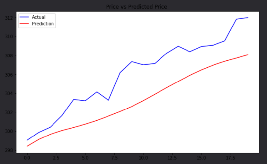
The algorithm we built to demonstrate how LSTM can be incorporated into QuantConnect is very simple. We used the model from the research environment and predicted the next price of SPY each day. Then, we emit Insights for inverse Treasury ETFs and SP500 Sector ETFs if the prediction is up, and we emit Insights for long Treasury ETFs if not. To do this we broke the algorithm up into a few methods. First, we built a scheduled event to train the model every month. Since this is a computationally-intensive operation, we wrapped the scheduled event in the Train() method.
# In Initialize
self.Train(self.DateRules.MonthEnd(), self.TimeRules.At(8,0), self.TrainMyModel)

def TrainMyModel(self):
    qb = self
    # Fetch history
    history = qb.History([symbol for key, symbol in self.macro_symbols.items()], 1280, Resolution.Daily)
    # Iterate over macro symbols
    for key, symbol in self.macro_symbols.items():
        # Initialize LSTM class instance lstm = MyLSTM()
        # Prepare data
        features_set, labels, training_data, test_data = lstm.ProcessData(history.loc[symbol].close)
        # Build model layers lstm.CreateModel(features_set, labels)
        # Fit model
        lstm.FitModel(features_set, labels)
        # Add LSTM class to dictionary to store later
        self.models[key] = lstm
Then, we built a predict function to make our predictions every day, 5-minutes after MarketOpen.
def Predict(self): delta = {} qb = self for key, symbol in self.macro_symbols.items(): # Fetch LSTM class lstm = self.models[key] # Fetch history history = qb.History([symbol for key, symbol in self.macro_symbols.items()], 80, Resolution.Daily) # Predict predictions = lstm.PredictFromModel(history.loc[symbol].close) # Grab latest prediction and calculate if predict symbol to go up or down delta[key] = ( predictions[-1] / self.Securities[symbol].Price ) - 1 # Plot prediction self.Plot('Prediction Plot', f'Predicted {key}', predictions[-1]) insights = [] # Iterate over macro symbols for key, change in delta.items(): if key == 'Bull': insights += [Insight.Price(symbol, timedelta(1), InsightDirection.Up if change > 0 else InsightDirection.Flat) for symbol in LiquidETFUniverse.SP500Sectors.Long if self.Securities.ContainsKey(symbol)] insights += [Insight.Price(symbol, timedelta(1), InsightDirection.Up if change > 0 else InsightDirection.Flat) for symbol in LiquidETFUniverse.Treasuries.Inverse if self.Securities.ContainsKey(symbol)] insights += [Insight.Price(symbol, timedelta(1), InsightDirection.Flat if change > 0 else InsightDirection.Up) for symbol in LiquidETFUniverse.Treasuries.Long if self.Securities.ContainsKey(symbol)] self.EmitInsights(insights)
Finally, we added a short method to plot the actual price vs the predicted price, which allows us to visually track what was happening in the algorithm.
def PlotMe(self): # Plot current price of symbols to match against prediction for key, symbol in self.macro_symbols.items(): self.Plot('Prediction Plot', f'Actual {key}', self.Securities[symbol].Price)
Since this is a computationally expensive algorithm, we used the Train() method, which allows for extended model-training without throwing a timeout error. This will be extremely useful for anyone looking to add ML methods to their algorithms, and you can find another example of this method here.Once the backtest runs, you can see that the model's predictions are fairly accurate considering the difficulties associated with modeling and predicting from a non-stationary series. It's not close enough for us to be able to claim to know the next SPY price at any given time, but it clearly gives sufficient information to inform us about market conditions at-large.


Alfred Aita
You imported but did not use MinMaxScaler. The results for this example would probably be the same.
Is this run on a GPU ? Just wondering
Liu Jin
Hi Sherry Yang , I've tried to run your algo on a longer time period (starting from 2015) but after about a year of backtest I get the error below. I would have thought that the Train() method ( https://github.com/QuantConnect/Lean/blob/master/Algorithm.Python/TrainingExampleAlgorithm.py ) would have solved this? What do you think? Thank you!
System.TimeoutException: Algorithm took longer than 10 minutes on a single time loop. CurrentTimeStepElapsed: 11.0 minutes
at QuantConnect.Isolator.MonitorTask (System.Threading.Tasks.Task task, System.TimeSpan timeSpan, System.Func`1[TResult] withinCustomLimits, System.Int64 memoryCap, System.Int32 sleepIntervalMillis) [0x002c4] in <eefa6b447f3a4e0eb61632434c9719a7>:0
at QuantConnect.Isolator.ExecuteWithTimeLimit (System.TimeSpan timeSpan, System.Func`1[TResult] withinCustomLimits, System.Action codeBlock, System.Int64 memoryCap, System.Int32 sleepIntervalMillis, QuantConnect.Util.WorkerThread workerThread) [0x00092] in <eefa6b447f3a4e0eb61632434c9719a7>:0
at QuantConnect.Lean.Engine.Engine.Run (QuantConnect.Packets.AlgorithmNodePacket job, QuantConnect.Lean.Engine.AlgorithmManager manager, System.String assemblyPath) [0x0099d] in <b0a99c0f99784925a4d272e02c8243cb>:0
Stanley Yang
great post!
I have tried to use other deep learning technique or LSTM in QC , but the problem is when you back testing longer than 3 to 5 years. you will get the following error message:(runtime error)
System.TimeoutException: Algorithm took longer than 10 minutes on a single time loop.
so I cannot file the algo in your alpha market, because your team ask for longer than 5 years backtesting record.
Alexandre Catarino
Hi!
Alfred Aita : MinMaxScaler is used in MyLSTM class' constructor. This is not run in GPU.
Liu Jin and Stanley Yang , did you try to play with the algorithm parameters? Maybe the neural networks model is taking too long to learn with 2015 conditions.
Please check out the docs, under Machine Learning, for more details on training limits.
Jack Simonson
Hey all,
Per a request from someone is support, we've created an example that uses a couple of technical indicators as features in an LSTM model. You can view the model in the research notebook attached below. Check it out, play with the inputs, and then find a way to put it into production!
Hyungjun Lim
Because the prediction is made on the raw value of the next day (as opposed to change amount) this tpye of predictoin when plotted, looks usually good.
But in fact, unless the daily price jump is of noticeable size, even prodicting no motion at all would still make the graph look decent, only that the graph is shifted by a day.
In order to correctly and faily display the prediction of time series, the plot should be done w.r.t the delta value, not the raw value.
Pangyuteng
This is a nice starting code to get our hands wets on neural nets.
Thank you for sharing Sherry. Very exciting!
I believe neural nets may be suitable for predicting trend, regime change and probably noise reduction. What I'm sharing below is doing none of the above! It is predicting next day stock return (!?) by feeding the LSTM with past Volatility Risk Premium (VRP, implied volatillity - historical volatility) and ratio of VIX and VXV (indication of Contago or Backwardation) [Tony Cooper, Easy Volatility Investing]. Custom data retreival is a copy pasta from Alex Muci's post "A simple VIX Strategy". I pretty much hacked through and crippled Sherry's code as this is just an excercise for me to get familiar with Quantconnect's framework and apis. The timeframe used here is cherry picked for a jolly PSR, training was done once as oppose to monthly, be wary of look ahead bias and other bugs. Expect timeout to occur if you enable monthly training and extend the backtesting timeframe.
Jared Broad
Nice work Ted! Worthy of its own discussion-thread if you were inclined.
That cherry-picking isn't so bad - we can call it tuned to "recent market behaviors".
The material on this website is provided for informational purposes only and does not constitute an offer to sell, a solicitation to buy, or a recommendation or endorsement for any security or strategy, nor does it constitute an offer to provide investment advisory services by QuantConnect. In addition, the material offers no opinion with respect to the suitability of any security or specific investment. QuantConnect makes no guarantees as to the accuracy or completeness of the views expressed in the website. The views are subject to change, and may have become unreliable for various reasons, including changes in market conditions or economic circumstances. All investments involve risk, including loss of principal. You should consult with an investment professional before making any investment decisions.
Dirk bothof
Hi guys, great resources!
This really inspired me to build some neural networks over the past weekend, however I feel that the current hardware underpinning QuantConnect is not suitable for this type of ML, a small net with relatively little input data (for a neural net) already has > 1 hour training time. To make something robust and value adding you need way more hardware.
It would be pretty great if I could add my own resources and pool that with the QuantConnect to speed things up or get access to a bigger pool of CPU's or a GPU at some extra fee. As is, I don't think it is feasible to do the propper research required, let alone trade neural net.
Does anybody have a different experience?
Best,
Dirk
Jared Broad
HI Dirk; professional subscriptions can harness more CPUs, and have a longer training period allocations for backtesting.
Live trading should be fine recalling a stored model, or retaining the previous models on a schedule as shown in the documentation above. It is happening in real-time which is 10000x slower than backtesting which should give it plenty of time to train the model to trade?
Adding a GPU backtesting option is a cool idea though and relatively easy for us to do. If there's demand we can test that out with the community. The GPU cards are expensive though it would need to be about $100/mo subscription to cover the hardware cost.
The material on this website is provided for informational purposes only and does not constitute an offer to sell, a solicitation to buy, or a recommendation or endorsement for any security or strategy, nor does it constitute an offer to provide investment advisory services by QuantConnect. In addition, the material offers no opinion with respect to the suitability of any security or specific investment. QuantConnect makes no guarantees as to the accuracy or completeness of the views expressed in the website. The views are subject to change, and may have become unreliable for various reasons, including changes in market conditions or economic circumstances. All investments involve risk, including loss of principal. You should consult with an investment professional before making any investment decisions.
Colton Surdyk
Couldn't you train the model offline on your own hardware and then load the saved model/weights manually in QC?
Jared Broad
You can train offline and load them into QC if you have the data - this would be fine for daily sources like Yahoo etc. For an intraday strategy that could be tricky.
We've created a new subscription upgrade "GPU Upgrade" - if we get >5 subscribers we'll add the necessary hardware. It's about $4,000 for the graphics card and there will be about 2-weeks setup time.
The material on this website is provided for informational purposes only and does not constitute an offer to sell, a solicitation to buy, or a recommendation or endorsement for any security or strategy, nor does it constitute an offer to provide investment advisory services by QuantConnect. In addition, the material offers no opinion with respect to the suitability of any security or specific investment. QuantConnect makes no guarantees as to the accuracy or completeness of the views expressed in the website. The views are subject to change, and may have become unreliable for various reasons, including changes in market conditions or economic circumstances. All investments involve risk, including loss of principal. You should consult with an investment professional before making any investment decisions.
Dirk bothof
Hi Jared,
Really cool to add GPU support this sets QC appart from competing platforms! For now I'm awaiting the L1 data to test my current stratgegies but will in parralel start reading on how to fully utilize the possibility of incorperating deep learning into a strategy!
Best,
Dirk
Antimarket
I've modified the code to run on the "EURUSD" and a set of other G10 currencies. The result is not satisfactory and it needs further exploration.
Thanks to Sherry Yang and Ted for the basic code implementation and Alexandre Catarino for his help.
Derek Melchin
Hi Apollos,
This algorithm's initialization process takes a while to complete because model training is computationally-intensive. Since we called the Train method, the algorithm can take up to 30 minutes to train the model before the backtest starts. To speed up the process, consider reducing the size of the neural network. For more information on model training, refer to our documentation.
Best,
Derek Melchin
The material on this website is provided for informational purposes only and does not constitute an offer to sell, a solicitation to buy, or a recommendation or endorsement for any security or strategy, nor does it constitute an offer to provide investment advisory services by QuantConnect. In addition, the material offers no opinion with respect to the suitability of any security or specific investment. QuantConnect makes no guarantees as to the accuracy or completeness of the views expressed in the website. The views are subject to change, and may have become unreliable for various reasons, including changes in market conditions or economic circumstances. All investments involve risk, including loss of principal. You should consult with an investment professional before making any investment decisions.
Apollos Hill
Hi Derek,
Thank you for the tip. I have been playing around with pytorch since then. Not sure why i didn't get your comment notification.
Shile Wen
Hi Baba Gi,
1. We may look into that for the future
2. This is one of the challenges of running LEAN locally. As a part of our agreement with our data providers, our data can't leave QuantConnect
3. Training periods are longer for higher level plans. If users are getting cut short, please contact our support at support@quantconnect.com
4. This is a good idea to explore.
One solution might be to train the models using less data but more periodically. Furthermore, if you could provide more details about your models, we might be able to give more suggestions on how to increase efficiency.
Best,
Shile Wen
AlMoJo
Hi everyone :)
I saw the backtest made by Pangyuteng and I have to say it looks amazing in terms of return / drawdown ratio.
When I tried to launch it I get this error message and nothing happens after the backtest starts launching.
Does anyone knows how to solve that please?
Thanks a lot
Vladimir
AlMoJo
Try changing in my_custom_data
url_vxv = "http://cache.quantconnect.com/alternative/cboe/vix3m.csv"url_vix = "http://cache.quantconnect.com/alternative/cboe/vix.csv"
Spacetime
AlMoJo ,
The data links for quandl were updated, so you will need to change the quandl data links in my_custom_data.py file
Please see the attached backtest project with the new quandl data links.
Hope that helps.
Quandl New Data Links:
https://cdn.cboe.com/api/global/us_indices/daily_prices/VIX_History.csv
https://cdn.cboe.com/api/global/us_indices/daily_prices/VIX3M_History.csv
Sherry Yang
The material on this website is provided for informational purposes only and does not constitute an offer to sell, a solicitation to buy, or a recommendation or endorsement for any security or strategy, nor does it constitute an offer to provide investment advisory services by QuantConnect. In addition, the material offers no opinion with respect to the suitability of any security or specific investment. QuantConnect makes no guarantees as to the accuracy or completeness of the views expressed in the website. The views are subject to change, and may have become unreliable for various reasons, including changes in market conditions or economic circumstances. All investments involve risk, including loss of principal. You should consult with an investment professional before making any investment decisions.
To unlock posting to the community forums please complete at least 30% of Boot Camp.
You can continue your Boot Camp training progress from the terminal. We hope to see you in the community soon!