Popular Libraries
Stable Baselines
Get Historical Data
Get some historical market data to train and test the model. For example, to get data for the different asset class ETFs during 2010 and 2023, run:
qb = QuantBook()
symbols = [
qb.add_equity("SPY", Resolution.DAILY).symbol,
qb.add_equity("GLD", Resolution.DAILY).symbol,
qb.add_equity("TLT", Resolution.DAILY).symbol,
qb.add_equity("USO", Resolution.DAILY).symbol,
qb.add_equity("UUP", Resolution.DAILY).symbol
]
df = qb.history(symbols, datetime(2010, 1, 1), datetime(2024, 1, 1))
Prepare Data
You need some historical data to prepare the data for the model. If you have historical data, manipulate it to train and test the model. In this example, extract the close price series as the outcome and obtain the partial-differenced time-series of OHLCV values as the observation.
history = df.unstack(0) # Select weight 0.5 here. Ideally, strike a balance between variance retained and stationarity. partial_diff = (history.diff() * 0.5 + history * 0.5).iloc[1:].fillna(0) history = history.close.iloc[1:]
Train Models
You need to prepare the historical data for training before you train the model. If you have prepared the data, build and train the environment and the model. In this example, create a gym environment to initialize the training environment, agent and reward. Then, create a RL model by DQN algorithm. Follow these steps to create the environment and the model:
- Split the data for training and testing to evaluate the model.
- Create a custom
gymenvironment class. - Initialize the environment.
- Train the model.
X_train = partial_diff.iloc[:-100].values X_test = partial_diff.iloc[-100:].values y_train = history.iloc[:-100].values y_test = history.iloc[-100:].values
In this example, create a custom environment with previous 5 OHLCV partial-differenced price data as the observation and the lowest maximum drawdown as the reward.
class PortfolioEnv(gym.Env):
def __init__(self, data, prediction, num_stocks):
super(PortfolioEnv, self).__init__()
self.data = data
self.prediction = prediction
self.num_stocks = num_stocks
self.current_step = 5
self.portfolio_value = []
self.portfolio_weights = np.ones(num_stocks) / num_stocks
# Define the action and observation spaces
self.action_space = gym.spaces.Box(low=-1.0, high=1.0, shape=(num_stocks, ), dtype=np.float32)
self.observation_space = gym.spaces.Box(low=-np.inf, high=np.inf, shape=(5, data.shape[1]))
def reset(self):
self.current_step = 5
self.portfolio_value = []
self.portfolio_weights = np.ones(self.num_stocks) / self.num_stocks
return self._get_observation()
def step(self, action):
# Normalize the portfolio weights
sum_weights = np.sum(np.abs(action))
if sum_weights > 1:
action /= sum_weights
# Deduct transaction fee
value = self.prediction[self.current_step]
fees = np.abs(self.portfolio_weights - action) @ value
# Update portfolio weights based on the chosen action
self.portfolio_weights = action
# Update portfolio value based on the new weights and the market prices less fee
self.portfolio_value.append(np.dot(self.portfolio_weights, value) - fees)
# Move to the next time step
self.current_step += 1
# Check if the episode is done (end of data)
done = self.current_step >= len(self.data) - 1
# Calculate the reward using max drawdown
reward = self._neg_max_drawdown
return self._get_observation(), reward, done, {}
def _get_observation(self):
# Return the last 5 partial differencing OHLCV as the observation
return self.data[self.current_step-5:self.current_step]
@property
def _neg_max_drawdown(self):
# Return max drawdown within 20 days in portfolio value as reward (negate since max reward is preferred)
portfolio_value_20d = np.array(self.portfolio_value[-min(len(self.portfolio_value), 20):])
acc_max = np.maximum.accumulate(portfolio_value_20d)
return -(portfolio_value_20d - acc_max).min()
def render(self, mode='human'):
# Implement rendering if needed
pass
# Initialize the environment env = PortfolioEnv(X_train, y_train, 5) # Wrap the environment in a vectorized environment env = DummyVecEnv([lambda: env]) # Normalize the observation space env = VecNormalize(env, norm_obs=True, norm_reward=False)
In this example, create a RL model and train with MLP-policy PPO algorithm.
# Define the PPO agent
model = PPO("MlpPolicy", env, verbose=0)
# Train the agent
model.learn(total_timesteps=100000)
Test Models
You need to build and train the model before you test its performance. If you have trained the model, test it on the out-of-sample data. Follow these steps to test the model:
- Initialize a return series to calculate performance and a list to store the equity value at each timestep.
- Iterate each testing data point for prediction and trading.
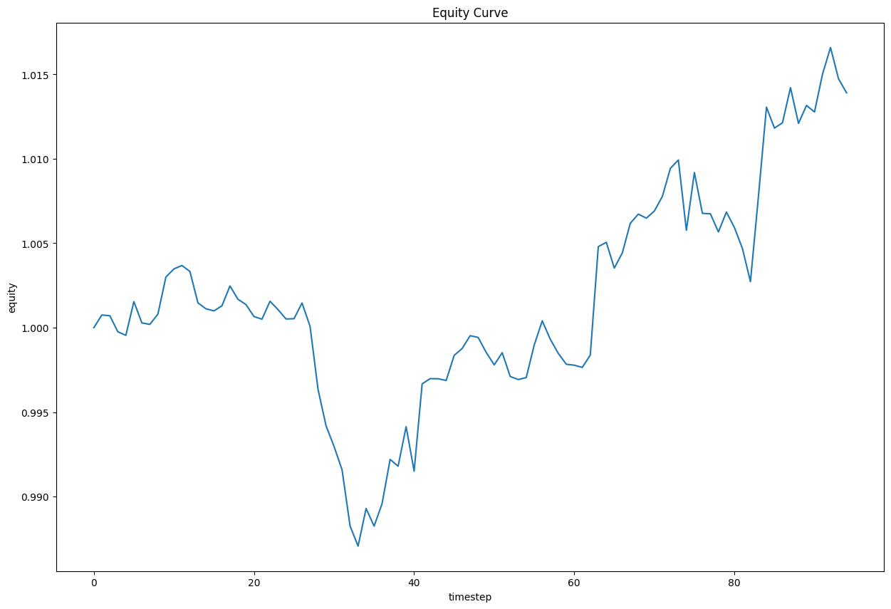
- Plot the result.
test = np.log(y_test[1:]/y_test[:-1]) equity = [1]
for i in range(5, X_test.shape[0]-1):
action, _ = model.predict(X_test[i-5:i], deterministic=True)
sum_weights = np.sum(np.abs(action))
if sum_weights > 1:
action /= sum_weights
value = test[i] @ action.T
equity.append((1+value) * equity[i-5])
plt.figure(figsize=(15, 10))
plt.title("Equity Curve")
plt.xlabel("timestep")
plt.ylabel("equity")
plt.plot(equity)
plt.show()
Store Models
You can save and load stable_baselines3 models using the Object Store.
Save Models
Follow these steps to save models in the Object Store:
- Set the key name of the model to be stored in the Object Store.
- Call the
GetFilePathget_file_pathmethod with the key. - Call the
savemethod with the file path.
model_key = "model"
file_name = qb.object_store.get_file_path(model_key)
This method returns the file path where the model will be stored.
model.save(file_name)
Load Models
You must save a model into the Object Store before you can load it from the Object Store. If you saved a model, follow these steps to load it:
- Call the
ContainsKeycontains_keymethod. - Call the
GetFilePathget_file_pathmethod with the key. - Call the
loadmethod with the file path, environment, and policy.
qb.object_store.contains_key(model_key)
This method returns a boolean that represents if the model_key is in the Object Store. If the Object Store does not contain the model_key, save the model using the model_key before you proceed.
file_name = qb.object_store.get_file_path(model_key)
This method returns the path where the model is stored.
loaded_model = PPO.load(file_name, env=env, policy="MlpPolicy")
This method returns the saved model.
Examples
The following examples demonstrate some common practices for using the stable_baselines3 library.
Example 1: Machine Trading
The following research notebook uses a stable_baselines3 machine learning model to make trading decisions, based on the previous 5 OHLCV partial differencing as observation.
# Import the gym and stable_baselines3 library.
import gym
from stable_baselines3 import PPO
from stable_baselines3.common.vec_env import DummyVecEnv, VecNormalize
# Instantiate the QuantBook for researching.
qb = QuantBook()
# Request the daily history with the date range to be studied.
symbols = [
qb.add_equity("SPY", Resolution.DAILY).symbol,
qb.add_equity("GLD", Resolution.DAILY).symbol,
qb.add_equity("TLT", Resolution.DAILY).symbol,
qb.add_equity("USO", Resolution.DAILY).symbol,
qb.add_equity("UUP", Resolution.DAILY).symbol
]
df = qb.history(symbols, datetime(2010, 1, 1), datetime(2024, 1, 1))
# Obtain the daily partial differencing to be the features and labels.
history = df.unstack(0)
# Select weight 0.5 here. Ideally, strike a balance between variance retained and stationarity.
partial_diff = (history.diff() * 0.5 + history * 0.5).iloc[1:].fillna(0)
history = history.close.iloc[1:]
# Split the data for training and testing to evaluate the model.
X_train = partial_diff.iloc[:-100].values
X_test = partial_diff.iloc[-100:].values
y_train = history.iloc[:-100].values
y_test = history.iloc[-100:].values
# Create a custom gym environment class. In this example, create a custom environment with previous 5 OHLCV partial-differenced price data as the observation and the lowest maximum drawdown as the reward.
class PortfolioEnv(gym.Env):
    def __init__(self, data, prediction, num_stocks):
        super(PortfolioEnv, self).__init__()

        self.data = data
        self.prediction = prediction
        self.num_stocks = num_stocks

        self.current_step = 5
        self.portfolio_value = []
        self.portfolio_weights = np.ones(num_stocks) / num_stocks

        # Define the action and observation spaces
        self.action_space = gym.spaces.Box(low=-1.0, high=1.0, shape=(num_stocks, ), dtype=np.float32)
        self.observation_space = gym.spaces.Box(low=-np.inf, high=np.inf, shape=(5, data.shape[1]))

    def reset(self):
        self.current_step = 5
        self.portfolio_value = []
        self.portfolio_weights = np.ones(self.num_stocks) / self.num_stocks

        return self._get_observation()

    def step(self, action):
        # Normalize the portfolio weights
        sum_weights = np.sum(np.abs(action))
        if sum_weights > 1:
            action /= sum_weights

        # Deduct transaction fee
        value = self.prediction[self.current_step]
        fees = np.abs(self.portfolio_weights - action) @ value

        # Update portfolio weights based on the chosen action
        self.portfolio_weights = action

        # Update portfolio value based on the new weights and the market prices less fee
        self.portfolio_value.append(np.dot(self.portfolio_weights, value) - fees)

        # Move to the next time step
        self.current_step += 1

        # Check if the episode is done (end of data)
        done = self.current_step >= len(self.data) - 1

        # Calculate the reward using max drawdown
        reward = self._neg_max_drawdown

        return self._get_observation(), reward, done, {}

    def _get_observation(self):
        # Return the last 5 partial differencing OHLCV as the observation
        return self.data[self.current_step-5:self.current_step]

    @property
    def _neg_max_drawdown(self):
        # Return max drawdown within 20 days in portfolio value as reward (negate since max reward is preferred)
        portfolio_value_20d = np.array(self.portfolio_value[-min(len(self.portfolio_value), 20):])
        acc_max = np.maximum.accumulate(portfolio_value_20d)
        return -(portfolio_value_20d - acc_max).min()

    def render(self, mode='human'):
        # Implement rendering if needed
        pass
# Initialize the environment.
env = PortfolioEnv(X_train, y_train, 5)
# Wrap the environment in a vectorized environment.
env = DummyVecEnv([lambda: env])
# Normalize the observation space.
env = VecNormalize(env, norm_obs=True, norm_reward=False)
# Train the model. In this example, create a RL model and train with MLP-policy PPO algorithm.
# Define the PPO agent.
model = PPO("MlpPolicy", env, verbose=0)
# Train the agent.
model.learn(total_timesteps=100000)
# Initialize a return series to calculate performance and a list to store the equity value at each timestep.
test = np.log(y_test[1:]/y_test[:-1])
equity = [1]
# Iterate each testing data point for prediction and trading.
for i in range(5, X_test.shape[0]-1):
    action, _ = model.predict(X_test[i-5:i], deterministic=True)
    sum_weights = np.sum(np.abs(action))
    if sum_weights > 1:
        action /= sum_weights
    value = test[i] @ action.T

    equity.append((1+value) * equity[i-5])
# Plot the result.
plt.figure(figsize=(15, 10))
plt.title("Equity Curve")
plt.xlabel("timestep")
plt.ylabel("equity")
plt.plot(equity)
plt.show()
# Store the model in the object store to allow accessing the model in the next research session or in the algorithm for trading.
model_key = "model"
file_name = qb.object_store.get_file_path(model_key)
model.save(file_name)
You can also see our Videos. You can also get in touch with us via Discord.
Did you find this page helpful?