Applying Research
PCA and Pairs Trading
Create Hypothesis
Principal Component Analysis (PCA) a way of mapping the existing dataset into a new "space", where the dimensions of the new data are linearly-independent, orthogonal vectors. PCA eliminates the problem of multicollinearity. In another way of thought, can we actually make use of the collinearity it implied, to find the collinear assets to perform pairs trading?
Import Libraries
We'll need to import libraries to help with data processing, validation and visualization. Import sklearn, arch, statsmodels, numpy and matplotlib libraries by the following:
from sklearn.decomposition import PCA
from arch.unitroot.cointegration import engle_granger
from statsmodels.tsa.stattools import adfuller
import numpy as np
from matplotlib import pyplot as plt
Get Historical Data
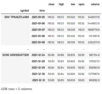
To begin, we retrieve historical data for researching.
- Instantiate a
QuantBook. - Select the desired tickers for research.
- Call the
add_equitymethod with the tickers, and their corresponding resolution. Then store theirSymbols. - Call the
historymethod withqb.securities.keysfor all tickers, time argument(s), and resolution to request historical data for the symbol.
qb = QuantBook()
symbols = {}
assets = ["SHY", "TLT", "SHV", "TLH", "EDV", "BIL",
          "SPTL", "TBT", "TMF", "TMV", "TBF", "VGSH", "VGIT",
          "VGLT", "SCHO", "SCHR", "SPTS", "GOVT"]
for i in range(len(assets)):
    symbols[assets[i]] = qb.add_equity(assets[i],Resolution.MINUTE).symbol
If you do not pass a resolution argument, Resolution.MINUTE is used by default.
history = qb.history(qb.securities.keys(), datetime(2021, 1, 1), datetime(2021, 12, 31), Resolution.DAILY)
Prepare Data
We'll have to process our data to get the principle component unit vector that explains the most variance, then find the highest- and lowest-absolute-weighing assets as the pair, since the lowest one's variance is mostly explained by the highest.
- Select the close column and then call the
unstackmethod. - Call
pct_changeto compute the daily return. - Initialize a
PCAmodel, then get the principle components by the maximum likelihood. - Get the number of principle component in a list, and their corresponding explained variance ratio.
- Plot the principle components' explained variance ratio.
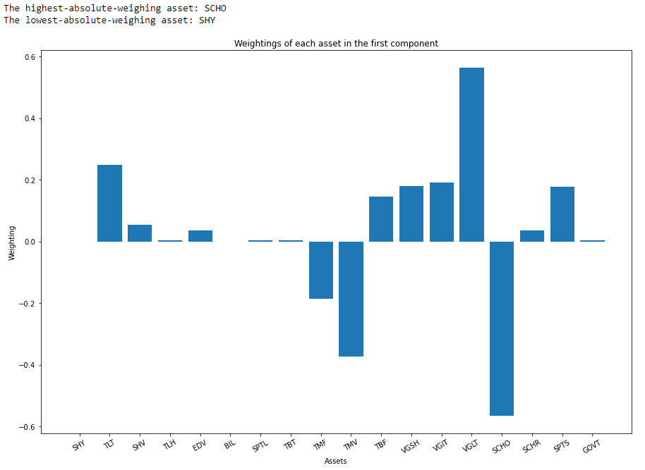
- Get the weighting of each asset in the first principle component.
- Select the highest- and lowest-absolute-weighing asset.
- Plot their weighings.
close_price = history['close'].unstack(level=0)
returns = close_price.pct_change().iloc[1:]
pca = PCA()
pca.fit(returns)
components = [str(x + 1) for x in range(pca.n_components_)]
explained_variance_pct = pca.explained_variance_ratio_ * 100
plt.figure(figsize=(15, 10))
plt.bar(components, explained_variance_pct)
plt.title("Ratio of Explained Variance")
plt.xlabel("Principle Component #")
plt.ylabel("%")
plt.show()
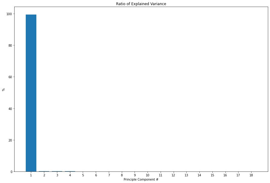
We can see over 95% of the variance is explained by the first principle. We could conclude that collinearity exists and most assets' return are correlated. Now, we can extract the 2 most correlated pairs.
first_component = pca.components_[0, :]
highest = assets[abs(first_component).argmax()]
lowest = assets[abs(first_component).argmin()]
print(f'The highest-absolute-weighing asset: {highest}\nThe lowest-absolute-weighing asset: {lowest}')
plt.figure(figsize=(15, 10))
plt.bar(assets, first_component)
plt.title("Weightings of each asset in the first component")
plt.xlabel("Assets")
plt.ylabel("Weighting")
plt.xticks(rotation=30)
plt.show()
Test Hypothesis
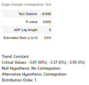
We now selected 2 assets as candidate for pair-trading. Hence, we're going to test if they are cointegrated and their spread is stationary to do so.
- Call
np.logto get the log price of the pair. - Test cointegration by Engle Granger Test.
- Get their cointegrating vector.
- Calculate the spread.
- Use Augmented Dickey Fuller test to test its stationarity.
- Plot the spread.
log_price = np.log(close_price[[highest, lowest]])
coint_result = engle_granger(log_price.iloc[:, 0], log_price.iloc[:, 1], trend="c", lags=0)
display(coint_result)
coint_vector = coint_result.cointegrating_vector[:2]
spread = log_price @ coint_vector
pvalue = adfuller(spread, maxlag=0)[1]
print(f"The ADF test p-value is {pvalue}, so it is {'' if pvalue < 0.05 else 'not '}stationary.")
spread.plot(figsize=(15, 10), title=f"Spread of {highest} and {lowest}")
plt.ylabel("Spread")
plt.show()
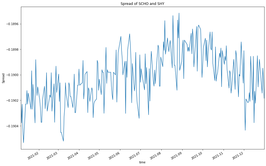
Result shown that the pair is cointegrated and their spread is stationary, so they are potential pair for pair-trading.
Set Up Algorithm
Pairs trading is exactly a 2-asset version of statistical arbitrage. Thus, we can just modify the algorithm from the Kalman Filter and Statistical Arbitrage tutorial, except we're using only a single cointegrating unit vector so no optimization of cointegration subspace is needed.
def initialize(self) -> None:

    #1. Required: Five years of backtest history
    self.set_start_date(2014, 1, 1)

    #2. Required: Alpha Streams Models:
    self.set_brokerage_model(BrokerageName.ALPHA_STREAMS)

    #3. Required: Significant AUM Capacity
    self.set_cash(1000000)

    #4. Required: Benchmark to SPY
    self.set_benchmark("SPY")

    self.assets = ["SCHO", "SHY"]

    # Add Equity ------------------------------------------------
    for i in range(len(self.assets)):
        self.add_equity(self.assets[i], Resolution.MINUTE).symbol

    # Instantiate our model
    self.recalibrate()

    # Set a variable to indicate the trading bias of the portfolio
    self.state = 0

    # Set Scheduled Event Method For Kalman Filter updating.
    self.schedule.on(self.date_rules.week_start(),
        self.time_rules.at(0, 0),
        self.recalibrate)

    # Set Scheduled Event Method For Kalman Filter updating.
    self.schedule.on(self.date_rules.every_day(),
        self.time_rules.before_market_close("SHY"),
        self.every_day_before_market_close)


def recalibrate(self) -> None:
    qb = self
    history = qb.history(self.assets, 252*2, Resolution.DAILY)
    if history.empty:
        return

    # Select the close column and then call the unstack method
    data = history['close'].unstack(level=0)

    # Convert into log-price series to eliminate compounding effect
    log_price = np.log(data)

    ### Get Cointegration Vectors
    # Get the cointegration vector
    coint_result = engle_granger(log_price.iloc[:, 0], log_price.iloc[:, 1], trend="c", lags=0)
    coint_vector = coint_result.cointegrating_vector[:2]

    # Get the spread
    spread = log_price @ coint_vector

    ### Kalman Filter
    # Initialize a Kalman Filter. Using the first 20 data points to optimize its initial state. We assume the market has no regime change so that the transitional matrix and observation matrix is [1].
    self.kalman_filter = KalmanFilter(transition_matrices = [1],
                        observation_matrices = [1],
                        initial_state_mean = spread.iloc[:20].mean(),
                        observation_covariance = spread.iloc[:20].var(),
                        em_vars=['transition_covariance', 'initial_state_covariance'])
    self.kalman_filter = self.kalman_filter.em(spread.iloc[:20], n_iter=5)
    (filtered_state_means, filtered_state_covariances) = self.kalman_filter.filter(spread.iloc[:20])

    # Obtain the current Mean and Covariance Matrix expectations.
    self.current_mean = filtered_state_means[-1, :]
    self.current_cov = filtered_state_covariances[-1, :]

    # Initialize a mean series for spread normalization using the Kalman Filter's results.
    mean_series = np.array([None]*(spread.shape[0]-20))

    # Roll over the Kalman Filter to obtain the mean series.
    for i in range(20, spread.shape[0]):
        (self.current_mean, self.current_cov) = self.kalman_filter.filter_update(filtered_state_mean = self.current_mean,
                                                                filtered_state_covariance = self.current_cov,
                                                                observation = spread.iloc[i])
        mean_series[i-20] = float(self.current_mean)

    # Obtain the normalized spread series.
    normalized_spread = (spread.iloc[20:] - mean_series)

    ### Determine Trading Threshold
    # Initialize 50 set levels for testing.
    s0 = np.linspace(0, max(normalized_spread), 50)

    # Calculate the profit levels using the 50 set levels.
    f_bar = np.array([None]*50)
    for i in range(50):
        f_bar[i] = len(normalized_spread.values[normalized_spread.values > s0[i]])               / normalized_spread.shape[0]

    # Set trading frequency matrix.
    D = np.zeros((49, 50))
    for i in range(D.shape[0]):
        D[i, i] = 1
        D[i, i+1] = -1

    # Set level of lambda.
    l = 1.0

    # Obtain the normalized profit level.
    f_star = np.linalg.inv(np.eye(50) + l * D.T@D) @ f_bar.reshape(-1, 1)
    s_star = [f_star[i]*s0[i] for i in range(50)]
    self.threshold = s0[s_star.index(max(s_star))]

    # Set the trading weight. We would like the portfolio absolute total weight is 1 when trading.
    self.trading_weight = coint_vector / np.sum(abs(coint_vector))


def every_day_before_market_close(self) -> None:
    qb = self

    # Get the real-time log close price for all assets and store in a Series
    series = pd.Series()
    for symbol in qb.securities.keys():
        series[symbol] = np.log(qb.securities[symbol].close)

    # Get the spread
    spread = np.sum(series * self.trading_weight)

    # Update the Kalman Filter with the Series
    (self.current_mean, self.current_cov) = self.kalman_filter.filter_update(filtered_state_mean = self.current_mean,
                                                                        filtered_state_covariance = self.current_cov,
                                                                        observation = spread)

    # Obtain the normalized spread.
    normalized_spread = spread - self.current_mean

    # ==============================

    # Mean-reversion
    if normalized_spread < -self.threshold:
        orders = []
        for i in range(len(self.assets)):
            orders.append(PortfolioTarget(self.assets[i], self.trading_weight[i]))
            self.set_holdings(orders)

        self.state = 1

    elif normalized_spread > self.threshold:
        orders = []
        for i in range(len(self.assets)):
            orders.append(PortfolioTarget(self.assets[i], -1 * self.trading_weight[i]))
            self.set_holdings(orders)

        self.state = -1

    # Out of position if spread recovered
    elif self.state == 1 and normalized_spread > -self.threshold or self.state == -1 and normalized_spread < self.threshold:
        self.liquidate()

        self.state = 0
Examples
The below code snippets concludes the above jupyter research notebook content.
from sklearn.decomposition import PCA
from arch.unitroot.cointegration import engle_granger
from statsmodels.tsa.stattools import adfuller

# Instantiate a QuantBook.
qb = QuantBook()

# Select the desired tickers for research.
assets = ["SHY", "TLT", "SHV", "TLH", "EDV", "BIL",
          "SPTL", "TBT", "TMF", "TMV", "TBF", "VGSH", "VGIT",
          "VGLT", "SCHO", "SCHR", "SPTS", "GOVT"]

# Call the AddEquity method with the tickers, and its corresponding resolution. Then store their Symbols. Resolution.Minute is used by default.
for i in range(len(assets)):
    qb.add_equity(assets[i],Resolution.MINUTE).symbol

# Call the History method with qb.Securities.Keys for all tickers, time argument(s), and resolution to request historical data for the symbol.
history = qb.history(qb.securities.keys(), datetime(2021, 1, 1), datetime(2021, 12, 31), Resolution.DAILY)

# Select the close column and then call the unstack method.
close_price = history['close'].unstack(level=0)

# Call pct_change to compute the daily return.
returns = close_price.pct_change().iloc[1:]

# Initialize a PCA model, then get the principle components by the maximum likelihood.
pca = PCA()
pca.fit(returns)

# Get the number of principle component in a list, and their corresponding explained variance ratio.
components = [str(x + 1) for x in range(pca.n_components_)]
explained_variance_pct = pca.explained_variance_ratio_ * 100

# Plot the principle components' explained variance ratio.
plt.figure(figsize=(15, 10))
plt.bar(components, explained_variance_pct)
plt.title("Ratio of Explained Variance")
plt.xlabel("Principle Component #")
plt.ylabel("%")
plt.show()

# Get the weighting of each asset in the first principle component.
first_component = pca.components_[0, :]

# Select the highest- and lowest-absolute-weighing asset.
highest = assets[abs(first_component).argmax()]
lowest = assets[abs(first_component).argmin()]
print(f'The highest-absolute-weighing asset: {highest}\nThe lowest-absolute-weighing asset: {lowest}')

# Plot their weighings.
plt.figure(figsize=(15, 10))
plt.bar(assets, first_component)
plt.title("Weightings of each asset in the first component")
plt.xlabel("Assets")
plt.ylabel("Weighting")
plt.xticks(rotation=30)
plt.show()

# Call np.log to get the log price of the pair.
log_price = np.log(close_price[[highest, lowest]])

# Test cointegration by Engle Granger Test.
coint_result = engle_granger(log_price.iloc[:, 0], log_price.iloc[:, 1], trend="c", lags=0)
display(coint_result)

# Get their cointegrating vector.
coint_vector = coint_result.cointegrating_vector[:2]

# Calculate the spread.
spread = log_price @ coint_vector

# Use Augmented Dickey Fuller test to test its stationarity.
pvalue = adfuller(spread, maxlag=0)[1]
print(f"The ADF test p-value is {pvalue}, so it is {'' if pvalue < 0.05 else 'not '}stationary.")

# Plot the spread.
spread.plot(figsize=(15, 10), title=f"Spread of {highest} and {lowest}")
plt.ylabel("Spread")
plt.show()
The below code snippets concludes the algorithm set up.
from arch.unitroot.cointegration import engle_granger
from pykalman import KalmanFilter

class PCADemo(QCAlgorithm):

    def initialize(self) -> None:
        self.set_start_date(2024, 9, 1)
        self.set_end_date(2024, 12, 31)
        self.set_cash(1000000)
        self.set_benchmark("SPY")
        self.assets = ["SCHO", "SHY"]

        # Add Equity ------------------------------------------------
        for i in range(len(self.assets)):
            self.add_equity(self.assets[i], Resolution.MINUTE).symbol

        # Instantiate our model
        self.recalibrate()

        # Set a variable to indicate the trading bias of the portfolio
        self.state = 0

        # Set Scheduled Event Method For Kalman Filter updating.
        self.schedule.on(self.date_rules.week_start(),
            self.time_rules.at(0, 0),
            self.recalibrate)

        # Set Scheduled Event Method For Kalman Filter updating.
        self.schedule.on(self.date_rules.every_day(),
            self.time_rules.before_market_close("SHY"),
            self.every_day_before_market_close)


    def recalibrate(self) -> None:
        qb = self
        history = qb.history(self.assets, 252*2, Resolution.DAILY)
        if history.empty: return

        # Select the close column and then call the unstack method
        data = history['close'].unstack(level=0)

        # Convert into log-price series to eliminate compounding effect
        log_price = np.log(data)

        ### Get Cointegration Vectors
        # Get the cointegration vector
        coint_result = engle_granger(log_price.iloc[:, 0], log_price.iloc[:, 1], trend="c", lags=0)
        coint_vector = coint_result.cointegrating_vector[:2]

        # Get the spread
        spread = log_price @ coint_vector

        ### Kalman Filter
        # Initialize a Kalman Filter. Using the first 20 data points to optimize its initial state. We assume the market has no regime change so that the transitional matrix and observation matrix is [1].
        self.kalman_filter = KalmanFilter(transition_matrices = [1],
                          observation_matrices = [1],
                          initial_state_mean = spread.iloc[:20].mean(),
                          observation_covariance = spread.iloc[:20].var(),
                          em_vars=['transition_covariance', 'initial_state_covariance'])
        self.kalman_filter = self.kalman_filter.em(spread.iloc[:20], n_iter=5)
        (filtered_state_means, filtered_state_covariances) = self.kalman_filter.filter(spread.iloc[:20])

        # Obtain the current Mean and Covariance Matrix expectations.
        self.current_mean = filtered_state_means[-1, :]
        self.current_cov = filtered_state_covariances[-1, :]

        # Initialize a mean series for spread normalization using the Kalman Filter's results.
        mean_series = np.array([None]*(spread.shape[0]-20))

        # Roll over the Kalman Filter to obtain the mean series.
        for i in range(20, spread.shape[0]):
            (self.current_mean, self.current_cov) = self.kalman_filter.filter_update(filtered_state_mean = self.current_mean,
                                                                   filtered_state_covariance = self.current_cov,
                                                                   observation = spread.iloc[i])
            mean_series[i-20] = float(self.current_mean)

        # Obtain the normalized spread series.
        normalized_spread = (spread.iloc[20:] - mean_series)

        ### Determine Trading Threshold
        # Initialize 50 set levels for testing.
        s0 = np.linspace(0, max(normalized_spread), 50)

        # Calculate the profit levels using the 50 set levels.
        f_bar = np.array([None]*50)
        for i in range(50):
            f_bar[i] = len(normalized_spread.values[normalized_spread.values > s0[i]])               / normalized_spread.shape[0]

        # Set trading frequency matrix.
        D = np.zeros((49, 50))
        for i in range(D.shape[0]):
            D[i, i] = 1
            D[i, i+1] = -1

        # Set level of lambda.
        l = 1.0

        # Obtain the normalized profit level.
        f_star = np.linalg.inv(np.eye(50) + l * D.T@D) @ f_bar.reshape(-1, 1)
        s_star = [f_star[i]*s0[i] for i in range(50)]
        self.threshold = s0[s_star.index(max(s_star))]

        # Set the trading weight. We would like the portfolio absolute total weight is 1 when trading.
        self.trading_weight = coint_vector / np.sum(abs(coint_vector))


    def every_day_before_market_close(self) -> None:
        qb = self

        # Get the real-time log close price for all assets and store in a Series
        series = pd.Series()
        for symbol in qb.securities.keys():
            series[symbol] = np.log(qb.securities[symbol].close)

        # Get the spread
        spread = np.sum(series * self.trading_weight)

        # Update the Kalman Filter with the Series
        (self.current_mean, self.current_cov) = self.kalman_filter.filter_update(filtered_state_mean = self.current_mean,
                                                                           filtered_state_covariance = self.current_cov,
                                                                           observation = spread)

        # Obtain the normalized spread.
        normalized_spread = spread - self.current_mean

        # ==============================

        # Mean-reversion
        if normalized_spread < -self.threshold:
            orders = []
            for i in range(len(self.assets)):
                orders.append(PortfolioTarget(self.assets[i], self.trading_weight[i]))
                self.set_holdings(orders)

            self.state = 1

        elif normalized_spread > self.threshold:
            orders = []
            for i in range(len(self.assets)):
                orders.append(PortfolioTarget(self.assets[i], -1 * self.trading_weight[i]))
                self.set_holdings(orders)

            self.state = -1

        # Out of position if spread recovered
        elif self.state == 1 and normalized_spread > -self.threshold or self.state == -1 and normalized_spread < self.threshold:
            self.liquidate()

            self.state = 0
You can also see our Videos. You can also get in touch with us via Discord.
Did you find this page helpful?