Applying Research
Long Short-Term Memory
Introduction
This page explains how to you can use the Research Environment to develop and test a Long Short Term Memory hypothesis, then put the hypothesis in production.
Recurrent neural networks (RNN) are a powerful tool in deep learning. These models quite accurately mimic how humans process sequencial information and learn. Unlike traditional feedforward neural networks, RNNs have memory. That is, information fed into them persists and the network is able to draw on this to make inferences.
Long Short-term Memory (LSTM) is a type of RNN. Instead of one layer, LSTM cells generally have four, three of which are part of "gates" -- ways to optionally let information through. The three gates are commonly referred to as the forget, input, and output gates. The forget gate layer is where the model decides what information to keep from prior states. At the input gate layer, the model decides which values to update. Finally, the output gate layer is where the final output of the cell state is decided. Essentially, LSTM separately decides what to remember and the rate at which it should update.
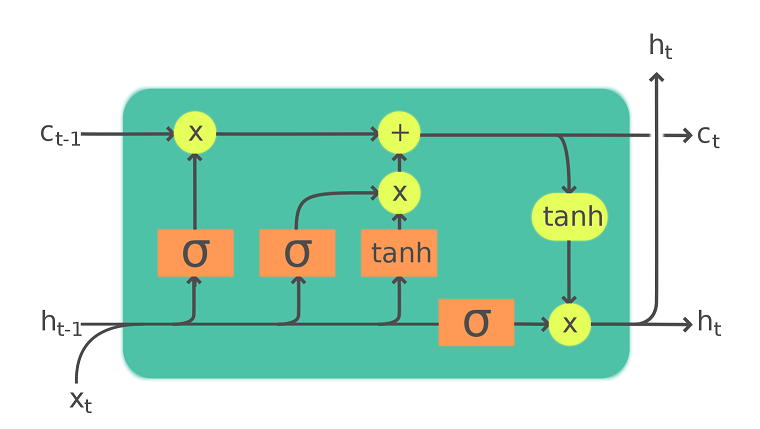
An exmaple of a LSTM cell: x is the input data, c is the long-term memory, h is the current state and serve as short-term memory, $\sigma$ and $tanh$ is the non-linear activation function of the gates.
Image source: https://en.wikipedia.org/wiki/Long_short-term_memory#/media/File:LSTM_Cell.svg
Create Hypothesis
LSTM models have produced some great results when applied to time-series prediction. One of the central challenges with conventional time-series models is that, despite trying to account for trends or other non-stationary elements, it is almost impossible to truly predict an outlier like a recession, flash crash, liquidity crisis, etc. By having a long memory, LSTM models are better able to capture these difficult trends in the data without suffering from the level of overfitting a conventional model would need in order to capture the same data.
For a very basic application, we're hypothesizing LSTM can offer an accurate prediction in future price.
Import Libraries
We'll need to import libraries to help with data processing, validation and visualization. Import keras, sklearn, numpy and matplotlib libraries by the following:
from keras.layers import LSTM, Dense, Dropout
from keras.models import Sequential
from keras.callbacks import EarlyStopping
from sklearn.preprocessing import MinMaxScaler

import numpy as np
from matplotlib import pyplot as plt
Get Historical Data
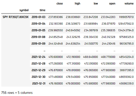
To begin, we retrieve historical data for researching.
- Instantiate a
QuantBook. - Select the desired index for research.
- Call the
add_equitymethod with the tickers, and their corresponding resolution. - Call the
historymethod withqb.securities.keysfor all tickers, time argument(s), and resolution to request historical data for the symbol.
qb = QuantBook()
asset = "SPY"
qb.add_equity(asset, Resolution.MINUTE)
If you do not pass a resolution argument, Resolution.MINUTE is used by default.
history = qb.history(qb.securities.keys(), datetime(2019, 1, 1), datetime(2021, 12, 31), Resolution.DAILY)
Prepare Data
We'll have to process our data as well as build the LSTM model before testing the hypothesis. We would scale our data to for better covergence.
- Select the close column and then call the
unstackmethod. - Initialize
MinMaxScalerto scale the data onto [0,1]. - Transform our data.
- Select input data
- Shift the data for 1-step backward as training output result.
- Split the data into training and testing sets.
- Build feauture and label sets (using number of steps 60, and feature rank 1).
close_price = history['close'].unstack(level=0)
scaler = MinMaxScaler(feature_range = (0, 1))
df = pd.DataFrame(scaler.fit_transform(close), index=close.index)
scaler = MinMaxScaler(feature_range = (0, 1))
output = df.shift(-1).iloc[:-1]
In this example, we use the first 80% data for trianing, and the last 20% for testing.
splitter = int(input_.shape[0] * 0.8)
X_train = input_.iloc[:splitter]
X_test = input_.iloc[splitter:]
y_train = output.iloc[:splitter]
y_test = output.iloc[splitter:]
features_set = []
labels = []
for i in range(60, X_train.shape[0]):
    features_set.append(X_train.iloc[i-60:i].values.reshape(-1, 1))
    labels.append(y_train.iloc[i])
features_set, labels = np.array(features_set), np.array(labels)
features_set = np.reshape(features_set, (features_set.shape[0], features_set.shape[1], 1))
Build Model
We construct the LSTM model.
- Build a
Sequentialkeras model. - Create the model infrastructure.
- Compile the model.
- Set early stopping callback method.
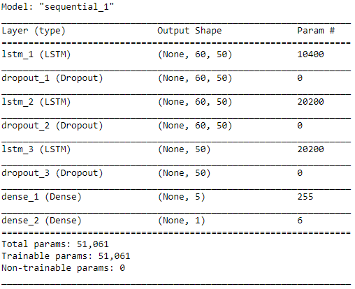
- Display the model structure.
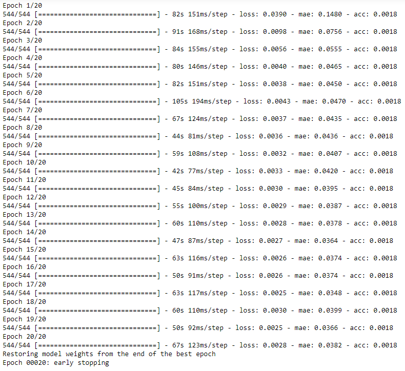
- Fit the model to our data, running 20 training epochs.
model = Sequential()
# Add our first LSTM layer - 50 nodes.
model.add(LSTM(units = 50, return_sequences=True, input_shape=(features_set.shape[1], 1)))
# Add Dropout layer to avoid overfitting
model.add(Dropout(0.2))
# Add additional layers
model.add(LSTM(units=50, return_sequences=True))
model.add(Dropout(0.2))
model.add(LSTM(units=50))
model.add(Dropout(0.2))
model.add(Dense(units = 5))
model.add(Dense(units = 1))
We use Adam as optimizer for adpative step size and MSE as loss function since it is continuous data.
model.compile(optimizer = 'adam', loss = 'mean_squared_error', metrics=['mae', 'acc'])
callback = EarlyStopping(monitor='loss', patience=3, verbose=1, restore_best_weights=True)
model.summary()
Note that different training session's results will not be the same since the batch is randomly selected.
model.fit(features_set, labels, epochs = 20, batch_size = 100, callbacks=[callback])
Test Hypothesis
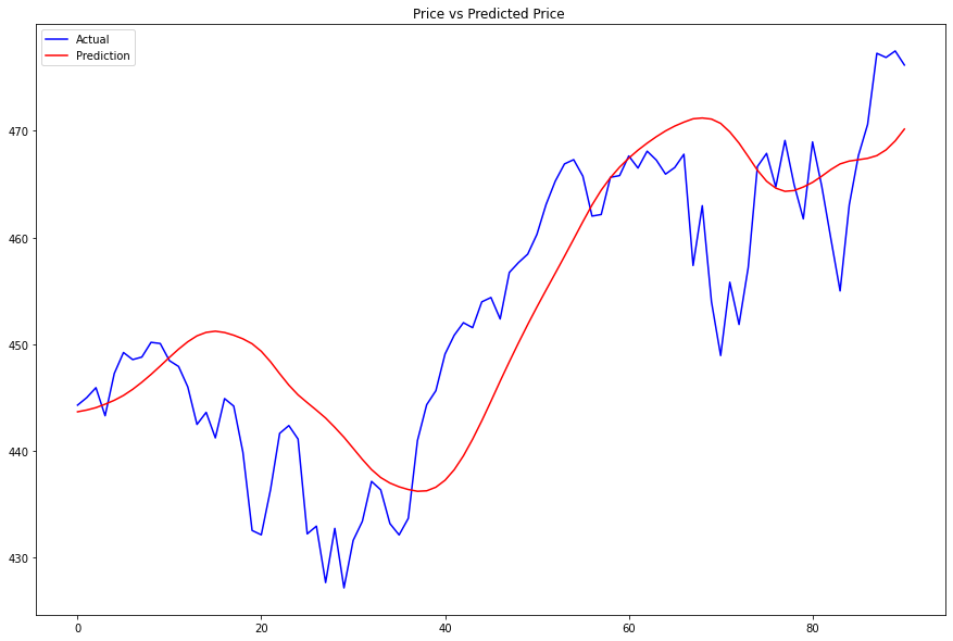
We would test the performance of this ML model to see if it could predict 1-step forward price precisely. To do so, we would compare the predicted and actual prices.
- Get testing set features for input.
- Make predictions.
- Transform predictions back to original data-scale.
- Plot the results.
test_features = []
for i in range(60, X_test.shape[0]):
    test_features.append(X_test.iloc[i-60:i].values.reshape(-1, 1))
test_features = np.array(test_features)
test_features = np.reshape(test_features, (test_features.shape[0], test_features.shape[1], 1))
predictions = model.predict(test_features)
predictions = scaler.inverse_transform(predictions)
actual = scaler.inverse_transform(y_test.values)
plt.figure(figsize=(15, 10))
plt.plot(actual[60:], color='blue', label='Actual')
plt.plot(predictions , color='red', label='Prediction')
plt.title('Price vs Predicted Price ')
plt.legend()
plt.show()
Set Up Algorithm
Once we are confident in our hypothesis, we can export this code into backtesting. One way to accomodate this model into backtest is to create a scheduled event which uses our model to predict the expected return. If we predict the price will go up, we long SPY, else, we short it.
def initialize(self) -> None:
    #1. Required: Five years of backtest history
    self.set_start_date(2016, 1, 1)

    #2. Required: Alpha Streams Models:
    self.set_brokerage_model(BrokerageName.ALPHA_STREAMS)

    #3. Required: Significant AUM Capacity
    self.set_cash(1000000)

    #4. Required: Benchmark to SPY
    self.set_benchmark("SPY")

    self.asset = "SPY"

    # Add Equity ------------------------------------------------
    self.add_equity(self.asset, Resolution.MINUTE)

    # Initialize the LSTM model
    self.build_model()

    # Set Scheduled Event Method For Our Model
    self.schedule.on(self.date_rules.every_day(),
        self.time_rules.before_market_close("SPY", 5),
        self.every_day_before_market_close)

    # Set Scheduled Event Method For Our Model Retraining every month
    self.schedule.on(self.date_rules.month_start(),
        self.time_rules.at(0, 0),
        self.build_model)
We'll also need to create a function to train and update our model from time to time.
def build_model(self) -> None:
    qb = self

    ### Preparing Data
    # Get historical data
    history = qb.history(qb.securities.keys(), 252*2, Resolution.DAILY)

    # Select the close column and then call the unstack method.
    close = history['close'].unstack(level=0)

    # Scale data onto [0,1]
    self.scaler = MinMaxScaler(feature_range = (0, 1))

    # Transform our data
    df = pd.DataFrame(self.scaler.fit_transform(close), index=close.index)

    # Feature engineer the data for input.
    input_ = df.iloc[1:]

    # Shift the data for 1-step backward as training output result.
    output = df.shift(-1).iloc[:-1]

    # Build feauture and label sets (using number of steps 60, and feature rank 1)
    features_set = []
    labels = []
    for i in range(60, input_.shape[0]):
        features_set.append(input_.iloc[i-60:i].values.reshape(-1, 1))
        labels.append(output.iloc[i])
    features_set, labels = np.array(features_set), np.array(labels)
    features_set = np.reshape(features_set, (features_set.shape[0], features_set.shape[1], 1))

    ### Build Model
    # Build a Sequential keras model
    self.model = Sequential()

    # Add our first LSTM layer - 50 nodes
    self.model.add(LSTM(units = 50, return_sequences=True, input_shape=(features_set.shape[1], 1)))
    # Add Dropout layer to avoid overfitting
    self.model.add(Dropout(0.2))
    # Add additional layers
    self.model.add(LSTM(units=50, return_sequences=True))
    self.model.add(Dropout(0.2))
    self.model.add(LSTM(units=50))
    self.model.add(Dropout(0.2))
    self.model.add(Dense(units = 5))
    self.model.add(Dense(units = 1))

    # Compile the model. We use Adam as optimizer for adpative step size and MSE as loss function since it is continuous data.
    self.model.compile(optimizer = 'adam', loss = 'mean_squared_error', metrics=['mae', 'acc'])

    # Set early stopping callback method
    callback = EarlyStopping(monitor='loss', patience=3, restore_best_weights=True)

    # Fit the model to our data, running 20 training epochs
    self.model.fit(features_set, labels, epochs = 20, batch_size = 1000, callbacks=[callback])
Now we export our model into the scheduled event method. We will switch qb with self and replace methods with their QCAlgorithm counterparts as needed. In this example, this is not an issue because all the methods we used in research also exist in QCAlgorithm.
def every_day_before_market_close(self) -> None:
    qb = self
    # Fetch history on our universe
    history = qb.history(qb.securities.keys(), 60, Resolution.DAILY)
    if history.empty:
        return

    # Make all of them into a single time index.
    close = history.close.unstack(level=0)

    # Scale our data
    df = pd.DataFrame(self.scaler.transform(close), index=close.index)

    # Feature engineer the data for input
    input_ = []
    input_.append(df.values.reshape(-1, 1))
    input_ = np.array(input_)
    input_ = np.reshape(input_, (input_.shape[0], input_.shape[1], 1))

    # Prediction
    prediction = self.model.predict(input_)

    # Revert the scaling into price
    prediction = self.scaler.inverse_transform(prediction)

    # ==============================

    if prediction > qb.securities[self.asset].price:
        self.set_holdings(self.asset, 1.)
    else:
        self.set_holdings(self.asset, -1.)
Examples
The below code snippets concludes the above jupyter research notebook content.
from keras.layers import LSTM, Dense, Dropout
from keras.models import Sequential
from keras.callbacks import EarlyStopping
from sklearn.preprocessing import MinMaxScaler

# Instantiate a QuantBook.
qb = QuantBook()

# Select the desired index for research.
asset = "SPY"
# Call the add_equity method with the tickers, and their corresponding resolution.
qb.add_equity(asset, Resolution.MINUTE)
# If you do not pass a resolution argument, Resolution.MINUTE is used by default.
# Call the history method with qb.securities.keys for all tickers, time argument(s), and resolution to request historical data for the symbol.
history = qb.history(qb.securities.keys(), datetime(2019, 1, 1), datetime(2021, 12, 31), Resolution.DAILY)

# Select the close column and then call the unstack method.
close_price = history['close'].unstack(level=0)
# Initialize MinMaxScaler to scale the data onto [0,1].
scaler = MinMaxScaler(feature_range = (0, 1))
# Transform our data.
df = pd.DataFrame(scaler.fit_transform(close), index=close.index)
# Select input data
scaler = MinMaxScaler(feature_range = (0, 1))
# Shift the data for 1-step backward as training output result.
output = df.shift(-1).iloc[:-1]
# Split the data into training and testing sets.
# In this example, we use the first 80% data for trianing, and the last 20% for testing.
splitter = int(input_.shape[0] * 0.8)
X_train = input_.iloc[:splitter]
X_test = input_.iloc[splitter:]
y_train = output.iloc[:splitter]
y_test = output.iloc[splitter:]
# Build feauture and label sets (using number of steps 60, and feature rank 1).
features_set = []
labels = []
for i in range(60, X_train.shape[0]):
    features_set.append(X_train.iloc[i-60:i].values.reshape(-1, 1))
    labels.append(y_train.iloc[i])
features_set, labels = np.array(features_set), np.array(labels)
features_set = np.reshape(features_set, (features_set.shape[0], features_set.shape[1], 1))

# Build a Sequential keras model.
model = Sequential()
# Create the model infrastructure.
# Add our first LSTM layer - 50 nodes.
model.add(LSTM(units = 50, return_sequences=True, input_shape=(features_set.shape[1], 1)))
# Add Dropout layer to avoid overfitting
model.add(Dropout(0.2))
# Add additional layers
model.add(LSTM(units=50, return_sequences=True))
model.add(Dropout(0.2))
model.add(LSTM(units=50))
model.add(Dropout(0.2))
model.add(Dense(units = 5))
model.add(Dense(units = 1))
# Compile the model. We use Adam as optimizer for adpative step size and MSE as loss function since it is continuous data.
model.compile(optimizer = 'adam', loss = 'mean_squared_error', metrics=['mae', 'acc'])
# Set early stopping callback method.
callback = EarlyStopping(monitor='loss', patience=3, verbose=1, restore_best_weights=True)
# Display the model structure.
model.summary()
# Fit the model to our data, running 20 training epochs.
# Note that different training session's results will not be the same since the batch is randomly selected.
model.fit(features_set, labels, epochs = 20, batch_size = 100, callbacks=[callback])

# Get testing set features for input.
test_features = []
for i in range(60, X_test.shape[0]):
    test_features.append(X_test.iloc[i-60:i].values.reshape(-1, 1))
test_features = np.array(test_features)
test_features = np.reshape(test_features, (test_features.shape[0], test_features.shape[1], 1))
# Make predictions.
predictions = model.predict(test_features)
# Transform predictions back to original data-scale.
predictions = scaler.inverse_transform(predictions)
actual = scaler.inverse_transform(y_test.values)
# Plot the results.
plt.figure(figsize=(15, 10))
plt.plot(actual[60:], color='blue', label='Actual')
plt.plot(predictions , color='red', label='Prediction')
plt.title('Price vs Predicted Price ')
plt.legend()
plt.show()
The below code snippets concludes the algorithm set up.
from keras.layers import LSTM, Dense, Dropout
from keras.models import Sequential
from keras.callbacks import EarlyStopping
from sklearn.preprocessing import MinMaxScaler

class LongShortTermMemoryAlgorithm(QCAlgorithm):
    def initialize(self) -> None:
        self.set_start_date(2024, 9, 1)
        self.set_end_date(2025, 12, 31)
        self.set_cash(1000000)
        self.set_benchmark("SPY")
        self.asset = "SPY"

        # Add Equity ------------------------------------------------
        self.add_equity(self.asset, Resolution.MINUTE)

        # Initialize the LSTM model
        self.build_model()

        # Set Scheduled Event Method For Our Model
        self.schedule.on(self.date_rules.every_day(),
            self.time_rules.before_market_close("SPY", 5),
            self.every_day_before_market_close)

        # Set Scheduled Event Method For Our Model Retraining every month
        self.schedule.on(self.date_rules.month_start(),
            self.time_rules.at(0, 0),
            self.build_model)

    def build_model(self) -> None:
        qb = self

        ### Preparing Data
        # Get historical data
        history = qb.history(qb.securities.keys(), 252*2, Resolution.DAILY)

        # Select the close column and then call the unstack method.
        close = history['close'].unstack(level=0)

        # Scale data onto [0,1]
        self.scaler = MinMaxScaler(feature_range = (0, 1))

        # Transform our data
        df = pd.DataFrame(self.scaler.fit_transform(close), index=close.index)

        # Feature engineer the data for input.
        input_ = df.iloc[1:]

        # Shift the data for 1-step backward as training output result.
        output = df.shift(-1).iloc[:-1]

        # Build feauture and label sets (using number of steps 60, and feature rank 1)
        features_set = []
        labels = []
        for i in range(60, input_.shape[0]):
            features_set.append(input_.iloc[i-60:i].values.reshape(-1, 1))
            labels.append(output.iloc[i])
        features_set, labels = np.array(features_set), np.array(labels)
        features_set = np.reshape(features_set, (features_set.shape[0], features_set.shape[1], 1))

        ### Build Model
        # Build a Sequential keras model
        self.model = Sequential()

        # Add our first LSTM layer - 50 nodes
        self.model.add(LSTM(units = 50, return_sequences=True, input_shape=(features_set.shape[1], 1)))
        # Add Dropout layer to avoid overfitting
        self.model.add(Dropout(0.2))
        # Add additional layers
        self.model.add(LSTM(units=50, return_sequences=True))
        self.model.add(Dropout(0.2))
        self.model.add(LSTM(units=50))
        self.model.add(Dropout(0.2))
        self.model.add(Dense(units = 5))
        self.model.add(Dense(units = 1))

        # Compile the model. We use Adam as optimizer for adpative step size and MSE as loss function since it is continuous data.
        self.model.compile(optimizer = 'adam', loss = 'mean_squared_error', metrics=['mae', 'acc'])

        # Set early stopping callback method
        callback = EarlyStopping(monitor='loss', patience=3, restore_best_weights=True)

        # Fit the model to our data, running 20 training epochs
        self.model.fit(features_set, labels, epochs = 20, batch_size = 1000, callbacks=[callback])

    def every_day_before_market_close(self) -> None:
        qb = self
        # Fetch history on our universe
        history = qb.history(qb.securities.keys(), 60, Resolution.DAILY)
        if history.empty:
            return

        # Make all of them into a single time index.
        close = history.close.unstack(level=0)

        # Scale our data
        df = pd.DataFrame(self.scaler.transform(close), index=close.index)

        # Feature engineer the data for input
        input_ = []
        input_.append(df.values.reshape(-1, 1))
        input_ = np.array(input_)
        input_ = np.reshape(input_, (input_.shape[0], input_.shape[1], 1))

        # Prediction
        prediction = self.model.predict(input_)

        # Revert the scaling into price
        prediction = self.scaler.inverse_transform(prediction)

        # ==============================

        if prediction > qb.securities[self.asset].price:
            self.set_holdings(self.asset, 1.)
        else:
            self.set_holdings(self.asset, -1.)
You can also see our Videos. You can also get in touch with us via Discord.
Did you find this page helpful?