Popular Libraries

Import the tensorflow and sklearn libraries.

import tensorflow as tf
from sklearn.model_selection import train_test_split

You need the sklearn library to prepare the data.

Get some historical market data to train and test the model. For example, to get data for the SPY ETF during 2020 and 2021, run:

qb = QuantBook()
symbol = qb.add_equity("SPY", Resolution.DAILY).symbol
history = qb.history(symbol, datetime(2020, 1, 1), datetime(2022, 1, 1)).loc[symbol]

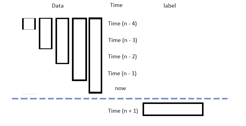
You need some historical data to prepare the data for the model. If you have historical data, manipulate it to train and test the model. In this example, use the following features and labels:

Follow these steps to prepare the data:

1. Loop through the DataFrame of historical prices and collect the features.

data = history

lookback = 5
lookback_series = []
for i in range(1, lookback + 1):
    df = data['close'].diff(i)[lookback:-1]
    df.name = f"close-{i}"
    lookback_series.append(df)
X = pd.concat(lookback_series, axis=1).reset_index(drop=True).dropna()
X

The following image shows the format of the features DataFrame:


2. Select the close column and then call the shift method to collect the labels.

Y = data['close'].diff(-1)

3. Drop the first 5 samples and then call the reset_index method.

Y = Y[lookback:-1].reset_index(drop=True)

This method aligns the history of the features and labels.

4. Split the data into training and testing datasets.

For example, to use the last third of data to test the model, run:

X_train, X_test, y_train, y_test = train_test_split(X.values, Y.values, test_size=0.33, shuffle=False)

You need to prepare the historical data for training before you train the model. If you have prepared the data, build and train the model. In this example, build a neural network model that predicts the future price of the SPY.

Build the Model

Follow these steps to build the model:

1. Set the number of layers, their number of nodes, the number of epochs, and the learning rate.

num_factors = X_test.shape[1]
num_neurons_1 = 10
num_neurons_2 = 10
num_neurons_3 = 5
epochs = 20
learning_rate = 0.0001

2. Create hidden layers with the set number of layers and their corresponding number of nodes.

This example uses the Keras API with ReLU activation for non-linear activation of each tensor.

model = tf.keras.Sequential([
    tf.keras.layers.Dense(num_neurons_1, activation=tf.nn.relu, input_shape=(num_factors,)),  # input shape required
    tf.keras.layers.Dense(num_neurons_2, activation=tf.nn.relu),
    tf.keras.layers.Dense(num_neurons_3, activation=tf.nn.relu),
    tf.keras.layers.Dense(1)
])

3. Select an optimizer.

This example uses the Adam optimizer. You can also use others like SGD.

optimizer = tf.keras.optimizers.Adam(learning_rate=learning_rate)

4. Define the loss function.

For numerical regression, use MSE as the objective function. For classification, cross entropy is more suitable.

def loss_mse(target_y, predicted_y):
    return tf.reduce_mean(tf.square(target_y - predicted_y))

Train the Model

Follow these steps to train the model:

1. Iteratively train the model over the set number of epochs. The model trains adaptively using the gradient from the loss function with the selected optimizer.

for i in range(epochs):
    with tf.GradientTape() as t:
        loss = loss_mse(y_train, model(X_train))

    train_loss = loss_mse(y_train, model(X_train))
    test_loss = loss_mse(y_test, model(X_test))
    print(f"""Epoch {i+1}:
Training loss = {train_loss.numpy()}. Test loss = {test_loss.numpy()}""")

    jac = t.gradient(loss, model.trainable_weights)
    optimizer.apply_gradients(zip(jac, model.trainable_weights))

You need to build and train the model before you test its performance. If you have trained the model, test it on the out-of-sample data. Follow these steps to test the model:

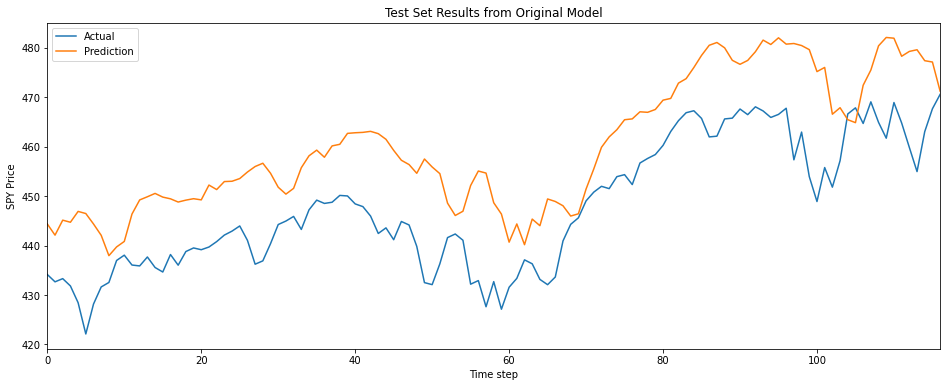
1. Create a helper function to plot the test set predictions on top of the SPY price.

def test_model(actual, title, X):
    prediction = model(X).numpy()
    prediction = prediction.reshape(-1, 1)

    plt.figure(figsize=(16, 6))
    plt.plot(actual, label="Actual")
    plt.plot(prediction, label="Prediction")
    plt.title(title)
    plt.xlabel("Time step")
    plt.ylabel("SPY Price")
    plt.legend()
    plt.show()

2. Call the helper function with the testing dataset.

test_model(y_test, "Test Set Results from Original Model", X_test)

You can save and load tensorflow models using the Object Store.

Save Models

Follow these steps to save models in the Object Store:

1. Set the key name of the model to be stored in the Object Store.

The key must end with a .keras extension for the native Keras format (recommended).

model_key = "model.keras"

2. Call the GetFilePathget_file_path method with the key.

file_name = qb.object_store.get_file_path(model_key)

This method returns the file path where the model will be stored.

3. Call the save method with the file path.

model.save(file_name)

4. Save the model to the Object Store.

qb.object_store.save(model_key)

Load Models

You must save a model into the Object Store before you can load it from the Object Store. If you saved a model, follow these steps to load it:

1. Call the GetFilePathget_file_path method with the key.

file_name = qb.object_store.get_file_path(model_key)

This method returns the path where the model is stored.

2. Call the load_model method with the file path.

model = tf.keras.models.load_model(file_name)

This method returns the saved model.

The following examples demonstrate some common practices for using the tensorflow library.

Example 1: Predict Next Return

The following research notebook uses a tensorflow machine learning model to predict the next day's return by the previous 5 days' close price differencing.

# Import the tensorflow library and others.
import tensorflow as tf
from sklearn.model_selection import train_test_split

# Instantiate the QuantBook for researching.
qb = QuantBook()
# Request the daily SPY history with the date range to be studied.
symbol = qb.add_equity("SPY", Resolution.DAILY).symbol
history = qb.history(symbol, datetime(2020, 1, 1), datetime(2022, 1, 1)).loc[symbol]

# Loop through the DataFrame of historical prices and collect the features.
data = history
lookback = 5
lookback_series = []
for i in range(1, lookback + 1):
    df = data['close'].diff(i)[lookback:-1]
    df.name = f"close-{i}"
    lookback_series.append(df)
X = pd.concat(lookback_series, axis=1).reset_index(drop=True).dropna()
# Select the close column and then call the shift method to collect the labels.
# This method aligns the history of the features and labels.
Y = data['close'].diff(-1)
Y = Y[lookback:-1].reset_index(drop=True)

# Split the data into training and testing datasets. For example, use the last third of data to test the model.
X_train, X_test, y_train, y_test = train_test_split(X.values, Y.values, test_size=0.33, shuffle=False)

# Set the number of layers, their number of nodes, the number of epochs, and the learning rate.
num_factors = X_test.shape[1]
num_neurons_1 = 10
num_neurons_2 = 10
num_neurons_3 = 5
epochs = 20
learning_rate = 0.0001
# Create hidden layers with the set number of layers and their corresponding number of nodes.
# This example uses the Keras API with ReLU activation for non-linear activation of each tensor.
model = tf.keras.Sequential([
    tf.keras.layers.Dense(num_neurons_1, activation=tf.nn.relu, input_shape=(num_factors,)),  # input shape required
    tf.keras.layers.Dense(num_neurons_2, activation=tf.nn.relu),
    tf.keras.layers.Dense(num_neurons_3, activation=tf.nn.relu),
    tf.keras.layers.Dense(1)
])
# This example uses the Adam optimizer. You can also use others like SGD.
optimizer = tf.keras.optimizers.Adam(learning_rate=learning_rate)
# Define the loss function. For numerical regression, use MSE as the objective function. For classification, cross entropy is more suitable.
def loss_mse(target_y, predicted_y):
    return tf.reduce_mean(tf.square(target_y - predicted_y))

# Iteratively train the model over the set number of epochs. The model trains adaptively using the gradient from the loss function with the selected optimizer.
for i in range(epochs):
    with tf.GradientTape() as t:
        loss = loss_mse(y_train, model(X_train))

    train_loss = loss_mse(y_train, model(X_train))
    test_loss = loss_mse(y_test, model(X_test))
    print(f"""Epoch {i+1}:
Training loss = {train_loss.numpy()}. Test loss = {test_loss.numpy()}""")

    jac = t.gradient(loss, model.trainable_weights)
    optimizer.apply_gradients(zip(jac, model.trainable_weights))

# Create a helper function to plot the test set predictions on top of the SPY price.
def test_model(actual, title, X):
    prediction = model(X).numpy()
    prediction = prediction.reshape(-1, 1)

    plt.figure(figsize=(16, 6))
    plt.plot(actual, label="Actual")
    plt.plot(prediction, label="Prediction")
    plt.title(title)
    plt.xlabel("Time step")
    plt.ylabel("SPY Price")
    plt.legend()
    plt.show()

test_model(y_test, "Test Set Results from Original Model", X_test)

# Store the model in the object store to allow accessing the model in the next research session or in the algorithm for trading.
model_key = "model.keras"
file_name = qb.object_store.get_file_path(model_key)
model.save(file_name)