Popular Libraries
Tslearn
Get Historical Data
Get some historical market data to train and test the model. For example, get data for the securities shown in the following table:
| Group Name | Tickers |
|---|---|
| Overall US market | SPY, QQQ, DIA |
| Tech companies | AAPL, MSFT, TSLA |
| Long-term US Treasury ETFs | IEF, TLT |
| Short-term US Treasury ETFs | SHV, SHY |
| Heavy metal ETFs | GLD, IAU, SLV |
| Energy sector | USO, XLE, XOM |
qb = QuantBook()
tickers = ["SPY", "QQQ", "DIA",
"AAPL", "MSFT", "TSLA",
"IEF", "TLT", "SHV", "SHY",
"GLD", "IAU", "SLV",
"USO", "XLE", "XOM"]
symbols = [qb.add_equity(ticker, Resolution.DAILY).symbol for ticker in tickers]
history = qb.history(symbols, datetime(2020, 1, 1), datetime(2022, 2, 20))
Prepare Data
You need some historical data to prepare the data for the model. If you have historical data, manipulate it to train and test the model. In this example, standardize the log close price time-series of the securities. Follow these steps to prepare the data:
- Unstack the historical DataFrame and select the close column.
- Take the logarithm of the historical time series.
- Standardize the data.
close = history.unstack(0).close
log_close = np.log(close)
Taking the logarithm eases the compounding effect.
standard_close = (log_close - log_close.mean()) / log_close.std()
Train Models
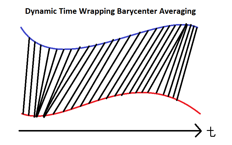
Instead of using real-time comparison, apply Dynamic Time Warping (DTW) with Barycenter Averaging (DBA). This technique averages multiple time-series into a single one without losing much of their information. Since not all time-series move efficiently as in ideal EMH assumptions, this approach enables similarity analysis of different time-series with sticky lags. Check the technical details from the tslearn documentation page.
Follow these steps to train the model:
- Set up the Time Series KMeans model with soft DBA.
- Call the
fitmethod with the prepared data.
km = TimeSeriesKMeans(n_clusters=6, # 6 main groups
metric="softdtw", # soft for differentiable
random_state=0)
km.fit(standard_close.T)
Test Models
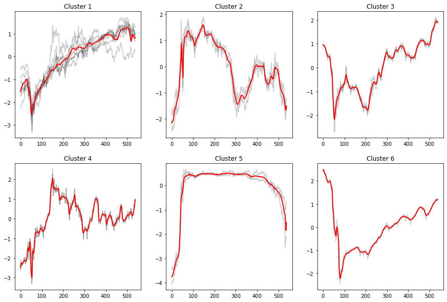
You need to build and train the model before you test its performance. If you have trained the model, visualize the clusters and their corresponding underlying series. Follow these steps to test the model:
- Call the
predictmethod with the data to get the cluster labels. - Create a helper function to plot the clusters.
- Plot the results.
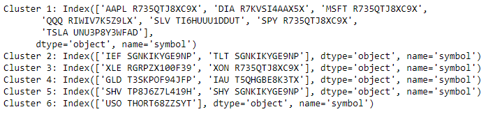
- Display the groupings.
labels = km.predict(standard_close.T)
def plot_helper(ts):
# Plot all points of the data set
for i in range(ts.shape[0]):
plt.plot(ts[i, :], "k-", alpha=.2)
# Plot the given barycenter of them
barycenter = softdtw_barycenter(ts, gamma=1.)
plt.plot(barycenter, "r-", linewidth=2)
j = 1
plt.figure(figsize=(15, 10))
for i in set(labels):
# Select the series in the i-th cluster.
X = standard_close.iloc[:, [n for n, k in enumerate(labels) if k == i]].values
# Plot the series and barycenter-averaged series.
plt.subplot(len(set(labels)) // 3 + (1 if len(set(labels))%3 != 0 else 0), 3, j)
plt.title(f"Cluster {i+1}")
plot_helper(X.T)
j += 1
plt.show()
for i in set(labels):
print(f"Cluster {i+1}: {standard_close.columns[[n for n, k in enumerate(labels) if k == i]]}")
Store Models
You can save and load tslearn models using the Object Store.
Save Models
Follow these steps to save models in the Object Store:
- Set the key name of the model to be stored in the Object Store.
- Call the
GetFilePathget_file_pathmethod with the key. - Delete the current file to avoid a
FileExistsErrorerror when you save the model. - Call the
to_hdf5method with the file path.
model_key = "model"
file_name = qb.object_store.get_file_path(model_key)
This method returns the file path where the model will be stored.
import os os.remove(file_name)
km.to_hdf5(file_name + ".hdf5")
Load Models
You must save a model into the Object Store before you can load it from the Object Store. If you saved a model, follow these steps to load it:
- Call the
ContainsKeycontains_keymethod. - Call the
GetFilePathget_file_pathmethod with the key. - Call the
from_hdf5method with the file path.
qb.object_store.contains_key(model_key)
This method returns a boolean that represents if the model_key is in the Object Store. If the Object Store does not contain the model_key, save the model using the model_key before you proceed.
file_name = qb.object_store.get_file_path(model_key)
This method returns the path where the model is stored.
loaded_model = TimeSeriesKMeans.from_hdf5(file_name + ".hdf5")
This method returns the saved model.
Examples
The following examples demonstrate some common practices for using the tslearn library.
Example 1: DBA Clustering
The following research notebook uses a tslearn machine learning model to cluster a collection of stocks applying Dynamic Time Warping (DTW) with Barycenter Averaging (DBA).
# Import the tslearn library.
from tslearn.barycenters import softdtw_barycenter
from tslearn.clustering import TimeSeriesKMeans
# Instantiate the QuantBook for researching.
qb = QuantBook()
# Request the daily history of the collection of stocks in the date range to be studied.
tickers = ["SPY", "QQQ", "DIA",
"AAPL", "MSFT", "TSLA",
"IEF", "TLT", "SHV", "SHY",
"GLD", "IAU", "SLV",
"USO", "XLE", "XOM"]
symbols = [qb.add_equity(ticker, Resolution.DAILY).symbol for ticker in tickers]
history = qb.history(symbols, datetime(2020, 1, 1), datetime(2022, 2, 20))
# Obtain the daily log close price to be analyzed.
close = history.unstack(0).close
log_close = np.log(close) # Taking the logarithm eases the compounding effect.
# Standardize the data for faster convergence.
standard_close = (log_close - log_close.mean()) / log_close.std()
# Set up the Time Series KMeans model with soft DBA.
km = TimeSeriesKMeans(n_clusters=6,   # 6 main groups
                      metric="softdtw",  # soft for differentiable
                      random_state=0)
# Fit the model.
km.fit(standard_close.T)
# Call the predict method with the data to get the cluster labels.
labels = km.predict(standard_close.T)
# Create a helper function to plot the clusters.
def plot_helper(ts):
    # Plot all points of the data set
    for i in range(ts.shape[0]):
        plt.plot(ts[i, :], "k-", alpha=.2)

    # Plot the given barycenter of them
    barycenter = softdtw_barycenter(ts, gamma=1.)
    plt.plot(barycenter, "r-", linewidth=2)
# Plot the results.
j = 1
plt.figure(figsize=(15, 10))
for i in set(labels):
    # Select the series in the i-th cluster.
    X = standard_close.iloc[:, [n for n, k in enumerate(labels) if k == i]].values

    # Plot the series and barycenter-averaged series.
    plt.subplot(len(set(labels)) // 3 + (1 if len(set(labels))%3 != 0 else 0), 3, j)
    plt.title(f"Cluster {i+1}")
    plot_helper(X.T)

    j += 1

plt.show()
# Display the groupings.
for i in set(labels):
    print(f"Cluster {i+1}: {standard_close.columns[[n for n, k in enumerate(labels) if k == i]]}")
# Store the model in the object store to allow accessing the model in the next research session or in the algorithm for trading.
model_key = "model"
file_name = qb.object_store.get_file_path(model_key)
import os
os.remove(file_name)
km.to_hdf5(file_name + ".hdf5")
You can also see our Videos. You can also get in touch with us via Discord.
Did you find this page helpful?