Applying Research
Hidden Markov Models
Create Hypothesis
A Markov process is a stochastic process where the possibility of switching to another state depends only on the current state of the model by the current state's probability distribution (it is usually represented by a state transition matrix). It is history-independent, or memoryless. While often a Markov process's state is observable, the states of a Hidden Markov Model (HMM) is not observable. This means the input(s) and output(s) are observable, but their intermediate, the state, is non-observable/hidden.
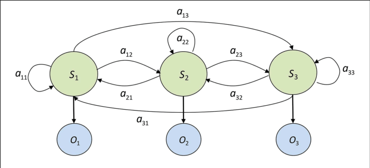
A 3-state HMM example, where S are the hidden states, O are the observable states and a are the probabilities of state transition.
Image source: Modeling Strategic Use of Human Computer Interfaces with Novel Hidden Markov Models. L. J. Mariano, et. al. (2015). Frontiers in Psychology 6:919. DOI:10.3389/fpsyg.2015.00919
In finance, HMM is particularly useful in determining the market regime, usually classified into "Bull" and "Bear" markets. Another popular classification is "Volatile" vs "Involatile" market, such that we can avoid entering the market when it is too risky. We hypothesis a HMM could be able to do the later, so we can produce a SPY-out-performing portfolio (positive alpha).
Import Libraries
We'll need to import libraries to help with data processing, validation and visualization. Import statsmodels, scipy, numpy, matplotlib and pandas libraries by the following:
from statsmodels.tsa.regime_switching.markov_regression import MarkovRegression
from scipy.stats import multivariate_normal
import numpy as np

from matplotlib import pyplot as plt
from pandas.plotting import register_matplotlib_converters
register_matplotlib_converters()
Get Historical Data
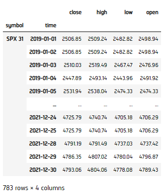
To begin, we retrieve historical data for researching.
- Instantiate a
QuantBook. - Select the desired index for research.
- Call the
add_indexmethod with the tickers, and their corresponding resolution. - Call the
historymethod withqb.securities.keysfor all tickers, time argument(s), and resolution to request historical data for the symbol.
qb = QuantBook()
asset = "SPX"
qb.add_index(asset, Resolution.MINUTE)
If you do not pass a resolution argument, Resolution.MINUTE is used by default.
history = qb.history(qb.securities.keys(), datetime(2019, 1, 1), datetime(2021, 12, 31), Resolution.DAILY)
Prepare Data
We'll have to process our data to get the volatility of the market for classification.
- Select the close column and then call the
unstackmethod. - Call
pct_changeto compute the daily return. - Initialize the HMM, then fit by the daily return data. Note that we're using varinace as switching regime, so
switching_varianceargument is set asTrue.
close_price = history['close'].unstack(level=0)
returns = close_price.pct_change().iloc[1:]
model = MarkovRegression(returns, k_regimes=2, switching_variance=True).fit()
display(model.summary())
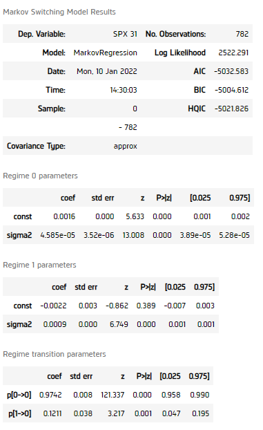
All p-values of the regime self-transition coefficients and the regime transition probability matrix's coefficient is smaller than 0.05, indicating the model should be able to classify the data into 2 different volatility regimes.
Test Hypothesis
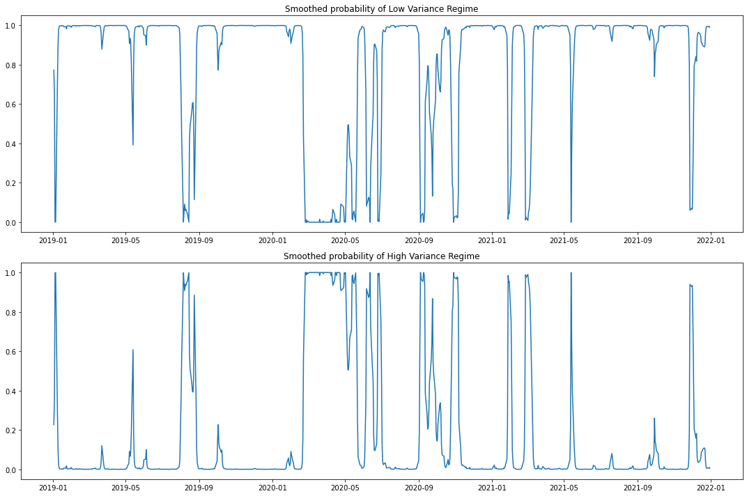
We now verify if the model can detect high and low volatility period effectively.
- Get the regime as a column, 1 as Low Variance Regime, 2 as High Variance Regime.
- Get the mean and covariance matrix of the 2 regimes, assume 0 covariance between the two.
- Fit a 2-dimensional multivariate normal distribution by the 2 means and covriance matrix.
- Get the normal distribution of each of the distribution.
- Plot the probability of data in different regimes.
- Plot the series into regime-wise.
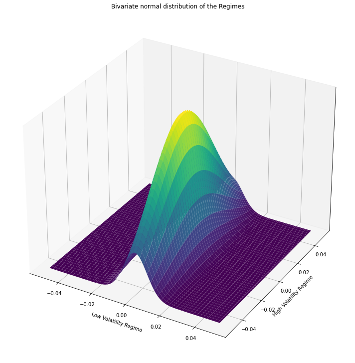
- Plot the distribution surface.
- Plot the contour.
regime = pd.Series(model.smoothed_marginal_probabilities.values.argmax(axis=1)+1,
                      index=returns.index, name='regime')
df_1 = close.loc[returns.index][regime == 1]
df_2 = close.loc[returns.index][regime == 2]
mean = np.array([returns.loc[df_1.index].mean(), returns.loc[df_2.index].mean()])
cov = np.array([[returns.loc[df_1.index].var(), 0], [0, returns.loc[df_2.index].var()]])
dist = multivariate_normal(mean=mean.flatten(), cov=cov)
mean_1, mean_2 = mean[0], mean[1]
sigma_1, sigma_2 = cov[0,0], cov[1,1]
x = np.linspace(-0.05, 0.05, num=100)
y = np.linspace(-0.05, 0.05, num=100)
X, Y = np.meshgrid(x,y)
pdf = np.zeros(X.shape)
for i in range(X.shape[0]):
    for j in range(X.shape[1]):
        pdf[i,j] = dist.pdf([X[i,j], Y[i,j]])
fig, axes = plt.subplots(2, figsize=(15, 10))
ax = axes[0]
ax.plot(model.smoothed_marginal_probabilities[0])
ax.set(title='Smoothed probability of Low Variance Regime')
ax = axes[1]
ax.plot(model.smoothed_marginal_probabilities[1])
ax.set(title='Smoothed probability of High Variance Regime')
fig.tight_layout()
plt.show()
df_1.index = pd.to_datetime(df_1.index)
df_1 = df_1.sort_index()
df_2.index = pd.to_datetime(df_2.index)
df_2 = df_2.sort_index()
plt.figure(figsize=(15, 10))
plt.scatter(df_1.index, df_1, color='blue', label="Low Variance Regime")
plt.scatter(df_2.index, df_2, color='red', label="High Variance Regime")
plt.title("Price series")
plt.ylabel("Price ($)")
plt.xlabel("Date")
plt.legend()
plt.show()
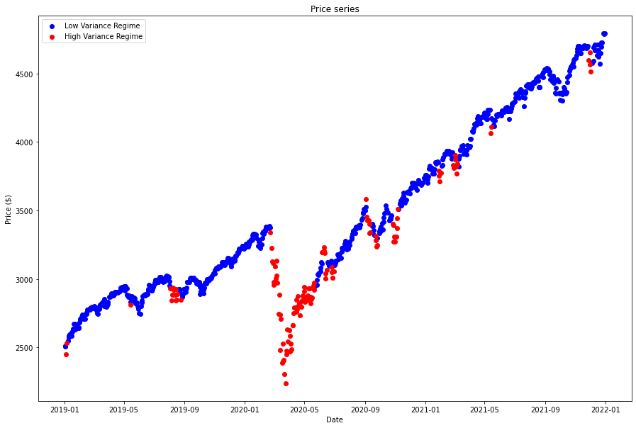
fig = plt.figure(figsize=(20, 10))
ax = fig.add_subplot(122, projection = '3d')
ax.plot_surface(X, Y, pdf, cmap = 'viridis')
ax.axes.zaxis.set_ticks([])
plt.xlabel("Low Volatility Regime")
plt.ylabel("High Volatility Regime")
plt.title('Bivariate normal distribution of the Regimes')
plt.tight_layout()
plt.show()
plt.figure(figsize=(12, 8))
plt.contourf(X, Y, pdf, cmap = 'viridis')
plt.xlabel("Low Volatility Regime")
plt.ylabel("High Volatility Regime")
plt.title('Bivariate normal distribution of the Regimes')
plt.tight_layout()
plt.show()
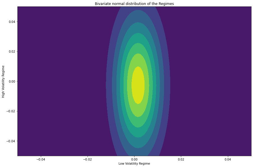
We can clearly seen from the results, the Low Volatility Regime has much lower variance than the High Volatility Regime, proven the model works.
Set Up Algorithm
Once we are confident in our hypothesis, we can export this code into backtesting. One way to accomodate this model into backtest is to create a scheduled event which uses our model to predict the expected return. Since we could calculate the expected return, we'd use Mean-Variance Optimization for portfolio construction.
def initialize(self) -> None:

    #1. Required: Five years of backtest history
    self.set_start_date(2008, 1, 1)
    self.set_end_date(2021, 1, 1)

    #2. Required: Alpha Streams Models:
    self.set_brokerage_model(BrokerageName.ALPHA_STREAMS)

    #3. Required: Significant AUM Capacity
    self.set_cash(1000000)

    #4. Required: Benchmark to SPY
    self.set_benchmark("SPY")

    self.assets = ["SPY", "TLT"]    # "TLT" as fix income in out-of-market period (high volatility)

    # Add Equity ------------------------------------------------
    for ticker in self.assets:
        self.add_equity(ticker, Resolution.MINUTE)

    # Set Scheduled Event Method For Kalman Filter updating.
    self.schedule.on(self.date_rules.every_day(),
        self.time_rules.before_market_close("SPY", 5),
        self.every_day_before_market_close)
Now we export our model into the scheduled event method. We will switch qb with self and replace methods with their QCAlgorithm counterparts as needed. In this example, this is not an issue because all the methods we used in research also exist in QCAlgorithm.
def every_day_before_market_close(self) -> None:
    qb = self

    # Get history
    history = qb.history(["SPY"], datetime(2010, 1, 1), datetime.now(), Resolution.DAILY)

    # Get the close price daily return.
    close = history['close'].unstack(level=0)

    # Call pct_change to obtain the daily return
    returns = close.pct_change().iloc[1:]

    # Initialize the HMM, then fit by the standard deviation data.
    model = MarkovRegression(returns, k_regimes=2, switching_variance=True).fit()

    # Obtain the market regime
    regime = model.smoothed_marginal_probabilities.values.argmax(axis=1)[-1]

    # ==============================

    if regime == 0:
        self.set_holdings([PortfolioTarget("TLT", 0.), PortfolioTarget("SPY", 1.)])
    else:
        self.set_holdings([PortfolioTarget("TLT", 1.), PortfolioTarget("SPY", 0.)])
Examples
The below code snippets concludes the above jupyter research notebook content.
from statsmodels.tsa.regime_switching.markov_regression import MarkovRegression
from scipy.stats import multivariate_normal
from pandas.plotting import register_matplotlib_converters
register_matplotlib_converters()

# Instantiate a QuantBook.
qb = QuantBook()

# Select the desired tickers for research.
asset = "SPX"

# Call the AddIndex method with the tickers, and its corresponding resolution. Then store their Symbols. Resolution.Minute is used by default.
qb.add_index(asset, Resolution.MINUTE)

# Call the history method with qb.securities.keys for all tickers, time argument(s), and resolution to request historical data for the symbol.
history = qb.history(qb.securities.keys(), datetime(2019, 1, 1), datetime(2021, 12, 31), Resolution.DAILY)

# Get the close price daily return.
close = history['close'].unstack(level=0)

# Call pct_change to obtain the daily return
returns = close.pct_change().iloc[1:]

# Initialize the HMM, then fit by the daily return data. Note that we're using varinace as switching regime, so switching_variance is set as True.
model = MarkovRegression(returns, k_regimes=2, switching_variance=True).fit()
display(model.summary())

# Get the regime as a column, 1 as Low Variance Regime, 2 as High Variance Regime.
regime = pd.Series(model.smoothed_marginal_probabilities.values.argmax(axis=1)+1,
                      index=returns.index, name='regime')
df_1 = close.loc[returns.index][regime == 1]
df_2 = close.loc[returns.index][regime == 2]

# Get the mean and covariance matrix of the 2 regimes, assume 0 covariance between the two.
mean = np.array([returns.loc[df_1.index].mean(), returns.loc[df_2.index].mean()])
cov = np.array([[returns.loc[df_1.index].var()[0], 0], [0, returns.loc[df_2.index].var()[0]]])

# Fit a 2-dimensional multivariate normal distribution by the 2 means and covriance matrix.
dist = multivariate_normal(mean=mean.flatten(), cov=cov)
mean_1, mean_2 = mean[0], mean[1]
sigma_1, sigma_2 = cov[0,0], cov[1,1]

# Get the normal distribution of each of the distribution.
x = np.linspace(-0.05, 0.05, num=100)
y = np.linspace(-0.05, 0.05, num=100)
X, Y = np.meshgrid(x,y)
pdf = np.zeros(X.shape)
for i in range(X.shape[0]):
    for j in range(X.shape[1]):
        pdf[i,j] = dist.pdf([X[i,j], Y[i,j]])

# Plot the probability of data in different regimes.
fig, axes = plt.subplots(2, figsize=(15, 10))
ax = axes[0]
ax.plot(model.smoothed_marginal_probabilities[0])
ax.set(title='Smoothed probability of Low Variance Regime')
ax = axes[1]
ax.plot(model.smoothed_marginal_probabilities[1])
ax.set(title='Smoothed probability of High Variance Regime')
fig.tight_layout()
plt.show()

# Plot the series into regime-wise.
df_1.index = pd.to_datetime(df_1.index)
df_1 = df_1.sort_index()
df_2.index = pd.to_datetime(df_2.index)
df_2 = df_2.sort_index()
plt.figure(figsize=(15, 10))
plt.scatter(df_1.index, df_1, color='blue', label="Low Variance Regime")
plt.scatter(df_2.index, df_2, color='red', label="High Variance Regime")
plt.title("Price series")
plt.ylabel("Price ($)")
plt.xlabel("Date")
plt.legend()
plt.show()

# Plot the distribution surface.
fig = plt.figure(figsize=(20, 10))
ax = fig.add_subplot(122, projection = '3d')
ax.plot_surface(X, Y, pdf, cmap = 'viridis')
ax.axes.zaxis.set_ticks([])
plt.xlabel("Low Volatility Regime")
plt.ylabel("High Volatility Regime")
plt.title('Bivariate normal distribution of the Regimes')
plt.tight_layout()
plt.show()

# plot the contour
plt.figure(figsize=(12, 8))
plt.contourf(X, Y, pdf, cmap = 'viridis')
plt.xlabel("Low Volatility Regime")
plt.ylabel("High Volatility Regime")
plt.title('Bivariate normal distribution of the Regimes')
plt.tight_layout()
plt.show()
The below code snippets concludes the algorithm set up.
from statsmodels.tsa.regime_switching.markov_regression import MarkovRegression

class HMMDemo(QCAlgorithm):
    def initialize(self):
        self.set_start_date(2024, 9, 1)
        self.set_end_date(2024, 12, 1)
        self.set_cash(1000000)
        self.set_benchmark("SPY")
        self.assets = ["SPY", "TLT"]    # "TLT" as fix income in out-of-market period (high volatility)

        # Add Equity ------------------------------------------------
        for ticker in self.assets:
            self.add_equity(ticker, Resolution.MINUTE).symbol

        # Set Scheduled Event Method For Kalman Filter updating.
        self.schedule.on(self.date_rules.every_day(),
            self.time_rules.before_market_close("SPY", 5),
            self.every_day_before_market_close)


    def every_day_before_market_close(self):
        qb = self

        # Get history
        history = qb.history(["SPY"], 252*3, Resolution.DAILY)

        # Get the close price daily return.
        close = history['close'].unstack(level=0)

        # Call pct_change to obtain the daily return
        returns = close.pct_change().iloc[1:]

        # Initialize the HMM, then fit by the standard deviation data.
        model = MarkovRegression(returns, k_regimes=2, switching_variance=True).fit()

        # Obtain the market regime
        regime = model.smoothed_marginal_probabilities.values.argmax(axis=1)[-1]

        # ==============================

        if regime == 0:
            self.set_holdings([PortfolioTarget("TLT", 0.), PortfolioTarget("SPY", 1.)])
        else:
            self.set_holdings([PortfolioTarget("TLT", 1.), PortfolioTarget("SPY", 0.)])
You can also see our Videos. You can also get in touch with us via Discord.
Did you find this page helpful?