Applying Research

We've assumed the price data is a time series with some auto regressive property (i.e. its expectation is related to past price information). Therefore, by using past information, we could predict the next price level. One way to do so is by Random Forest Regression, which is a supervised machine learning algorithm where its weight and bias is decided in non-linear hyperdimension.

We'll need to import libraries to help with data processing and machine learning. Import sklearn, numpy and matplotlib libraries by the following:

from sklearn.ensemble import RandomForestRegressor
import numpy as np
from matplotlib import pyplot as plt

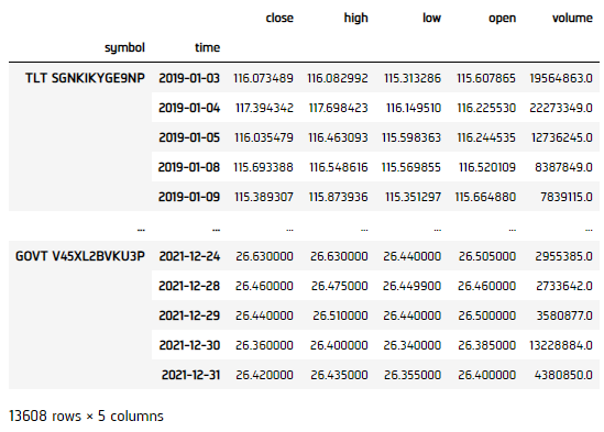
To begin, we retrieve historical data for researching.

1. Instantiate a QuantBook.

qb = QuantBook()

2. Select the desired tickers for research.

symbols = {}
assets = ["SHY", "TLT", "SHV", "TLH", "EDV", "BIL",
          "SPTL", "TBT", "TMF", "TMV", "TBF", "VGSH", "VGIT",
          "VGLT", "SCHO", "SCHR", "SPTS", "GOVT"]

3. Call the AddEquityadd_equity method with the tickers, and their corresponding resolution. Then store their Symbols.

for i in range(len(assets)):
    symbols[assets[i]] = qb.add_equity(assets[i],Resolution.MINUTE).symbol

If you do not pass a resolution argument, Resolution.MinuteResolution.MINUTE is used by default.

4. Call the Historyhistory method with qb.Securities.Keysqb.securities.keys for all tickers, time argument(s), and resolution to request historical data for the symbol.

history = qb.history(qb.securities.keys, datetime(2019, 1, 1), datetime(2021, 12, 31), Resolution.DAILY)

We'll have to process our data as well as to build the ML model before testing the hypothesis. Our methodology is to use fractional differencing close price as the input data in order to (1) provide stationarity, and (2) retain sufficient extent of variance of the previous price information. We assume d=0.5 is the right balance to do so.

1. Select the close column and then call the unstack method.

df = history['close'].unstack(level=0)

2. Feature engineer the data as fractional differencing for input.

input_ = df.diff() * 0.5 + df * 0.5
input_ = input_.iloc[1:]

3. Shift the data for 1-step backward as training output result.

output = df.shift(-1).iloc[:-1]

4. Split the data into training and testing sets.

splitter = int(input_.shape[0] * 0.8)
X_train = input_.iloc[:splitter]
X_test = input_.iloc[splitter:]
y_train = output.iloc[:splitter]
y_test = output.iloc[splitter:]

5. Initialize a Random Forest Regressor.

regressor = RandomForestRegressor(n_estimators=100, min_samples_split=5, random_state = 1990)

6. Fit the regressor.

regressor.fit(X_train, y_train)

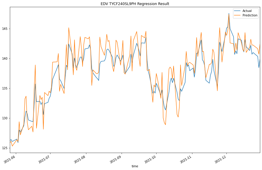
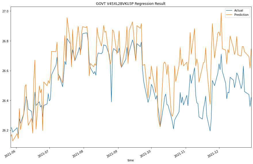
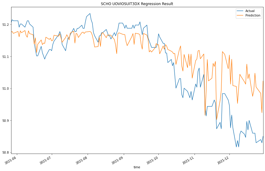
We would test the performance of this ML model to see if it could predict 1-step forward price precisely. To do so, we would compare the predicted and actual prices.

1. Predict the testing set.

predictions = regressor.predict(X_test)

2. Convert result into DataFrame.

predictions = pd.DataFrame(predictions, index=y_test.index, columns=y_test.columns)

3. Plot the result for comparison.

for col in y_test.columns:
    plt.figure(figsize=(15, 10))

    y_test[col].plot(label="Actual")
    predictions[col].plot(label="Prediction")

    plt.title(f"{col} Regression Result")
    plt.legend()
    plt.show()
    plt.clf()



For more plots, please clone the project and run the notebook.

Once we are confident in our hypothesis, we can export this code into backtesting. One way to accomodate this model into backtest is to create a scheduled event which uses our model to predict the expected return. Since we could calculate the expected return, we'd use Mean-Variance Optimization for portfolio construction.

def initialize(self) -> None:

    #1. Required: Five years of backtest history
    self.set_start_date(2014, 1, 1)

    #2. Required: Alpha Streams Models:
    self.set_brokerage_model(BrokerageName.ALPHA_STREAMS)

    #3. Required: Significant AUM Capacity
    self.set_cash(1000000)

    #4. Required: Benchmark to SPY
    self.set_benchmark("SPY")
    
    self.set_portfolio_construction(MeanVarianceOptimizationPortfolioConstructionModel(portfolio_bias = PortfolioBias.LONG,
                                                                                    period=252))
    self.set_execution(ImmediateExecutionModel())

    self.assets = ["SHY", "TLT", "IEI", "SHV", "TLH", "EDV", "BIL",
                    "SPTL", "TBT", "TMF", "TMV", "TBF", "VGSH", "VGIT",
                    "VGLT", "SCHO", "SCHR", "SPTS", "GOVT"]
    
    # Add Equity ------------------------------------------------ 
    for i in range(len(self.assets)):
        self.add_equity(self.assets[i], Resolution.MINUTE)
        
    # Initialize the timer to train the Machine Learning model
    self.time = datetime.min
    
    # Set Scheduled Event Method For Our Model
    self.schedule.on(self.date_rules.every_day(), self.time_rules.before_market_close("SHY", 5), self.every_day_before_market_close)

We'll also need to create a function to train and update our model from time to time.

def build_model(self) -> None:
    # Initialize the Random Forest Regressor
    self.regressor = RandomForestRegressor(n_estimators=100, min_samples_split=5, random_state = 1990)
    
    # Get historical data
    history = self.history(self.securities.keys, 360, Resolution.DAILY)
    
    # Select the close column and then call the unstack method.
    df = history['close'].unstack(level=0)
    
    # Feature engineer the data for input.
    input_ = df.diff() * 0.5 + df * 0.5
    input_ = input_.iloc[1:].ffill().fillna(0)
    
    # Shift the data for 1-step backward as training output result.
    output = df.shift(-1).iloc[:-1].ffill().fillna(0)
    
    # Fit the regressor
    self.regressor.fit(input_, output)

Now we export our model into the scheduled event method. We will switch qb with self and replace methods with their QCAlgorithm counterparts as needed. In this example, this is not an issue because all the methods we used in research also exist in QCAlgorithm.

def EveryDayBeforeMarketClose(self) -> None:
    # Retrain the regressor every month
    if self.time < self.Time:
        self.BuildModel()
        self.time = Expiry.EndOfMonth(self.Time)
    
    qb = self
    # Fetch history on our universe
    df = qb.History(qb.Securities.Keys, 2, Resolution.Daily)
    if df.empty: return

    # Make all of them into a single time index.
    df = df.close.unstack(level=0)

    # Feature engineer the data for input
    input_ = df.diff() * 0.5 + df * 0.5
    input_ = input_.iloc[-1].fillna(0).values.reshape(1, -1)
    
    # Predict the expected price
    predictions = self.regressor.predict(input_)
    
    # Get the expected return
    predictions = (predictions - df.iloc[-1].values) / df.iloc[-1].values
    predictions = predictions.flatten()

    # ==============================
    
    insights = []
    
    for i in range(len(predictions)):
        insights.append( Insight.Price(self.assets[i], timedelta(days=1), InsightDirection.Up, predictions[i]) )

    self.EmitInsights(insights)