Indicators

You need to subscribe to some market data in order to calculate indicator values.

var qb = new QuantBook();
var symbol = qb.AddEquity("SPY").Symbol;

qb = QuantBook()
symbol = qb.add_equity("SPY").symbol

You need to subscribe to some market data and create an indicator in order to calculate a timeseries of indicator values.

Follow these steps to create an indicator timeseries:

1. Get some historical data.

// Request historical trading data with the daily resolution.
var history = qb.History(symbol, 70, Resolution.Daily);

# Request historical trading data with the daily resolution.
history = qb.history[TradeBar](symbol, 70, Resolution.DAILY)

2. Create a data-point indicator.

In this example, use a 20-period 2-standard-deviation BollingerBands indicator.

var bb = new BollingerBands(20, 2);

bb = BollingerBands(20, 2)

3. Create a RollingWindow for each attribute of the indicator to hold their values.

// Create a window dictionary to store RollingWindow objects.
var window = new Dictionary<string, RollingWindow<decimal>>();
// Store the RollingWindow objects, index by key is the property of the indicator.
var time = new RollingWindow<DateTime>(50);
window["bollingerbands"] = new RollingWindow<decimal>(50);
window["lowerband"] = new RollingWindow<decimal>(50);
window["middleband"] = new RollingWindow<decimal>(50);
window["upperband"] = new RollingWindow<decimal>(50);
window["bandwidth"] = new RollingWindow<decimal>(50);
window["percentb"] = new RollingWindow<decimal>(50);
window["standarddeviation"] = new RollingWindow<decimal>(50);
window["price"] = new RollingWindow<decimal>(50);

# Create a window dictionary to store RollingWindow objects.
window = {}
# Store the RollingWindow objects, index by key is the property of the indicator.
window['time'] = RollingWindow[DateTime](50)
window["bollingerbands"] = RollingWindow[float](50)
window["lowerband"] = RollingWindow[float](50)
window["middleband"] = RollingWindow[float](50)
window["upperband"] = RollingWindow[float](50)
window["bandwidth"] = RollingWindow[float](50)
window["percentb"] = RollingWindow[float](50)
window["standarddeviation"] = RollingWindow[float](50)
window["price"] = RollingWindow[float](50)

4. Attach a handler method to the indicator that updates the RollingWindow objects.

// Define an update function to add the indicator values to the RollingWindow object.
bb.Updated += (sender, updated) => 
{
    var indicator = (BollingerBands)sender;
    time.Add(updated.EndTime);
    window["bollingerbands"].Add(updated);
    window["lowerband"].Add(indicator.LowerBand);
    window["middleband"].Add(indicator.MiddleBand);
    window["upperband"].Add(indicator.UpperBand);
    window["bandwidth"].Add(indicator.BandWidth);
    window["percentb"].Add(indicator.PercentB);
    window["standarddeviation"].Add(indicator.StandardDeviation);
    window["price"].Add(indicator.Price);
};

# Define an update function to add the indicator values to the RollingWindow object.
def update_bollinger_band_window(sender: object, updated: IndicatorDataPoint) -> None:
    indicator = sender
    window['time'].add(updated.end_time)
    window["bollingerbands"].add(updated.value)
    window["lowerband"].add(indicator.lower_band.current.value)
    window["middleband"].add(indicator.middle_band.current.value)
    window["upperband"].add(indicator.upper_band.current.value)
    window["bandwidth"].add(indicator.band_width.current.value)
    window["percentb"].add(indicator.percent_b.current.value)
    window["standarddeviation"].add(indicator.standard_deviation.current.value)
    window["price"].add(indicator.price.current.value)

bb.updated += UpdateBollingerBandWindow

When the indicator receives new data, the preceding handler method adds the new IndicatorDataPoint values into the respective RollingWindow.

5. Create a TradeBarConsolidator to consolidate data into the custom resolution.

var consolidator = new TradeBarConsolidator(TimeSpan.FromDays(7));

consolidator = TradeBarConsolidator(timedelta(days=7))

6. Attach a handler method to feed data into the consolidator and updates the indicator with the consolidated bars.

consolidator.DataConsolidated += (sender, consolidated) =>
{
    bb.Update(consolidated.EndTime, consolidated.Close);
};

def on_data_consolidated(sender, consolidated):
    bb.update(consolidated.end_time, consolidated.close)
consolidator.data_consolidated += on_data_consolidated

When the consolidator receives 7 days of data, the handler generates a 7-day TradeBar and update the indicator.

7. Iterate through the historical market data and update the indicator.

foreach(var bar in history)
{
    consolidator.Update(bar);
}

for bar in history:
    consolidator.update(bar)

8. Display the data.

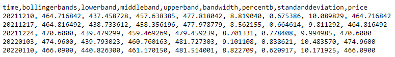
Console.WriteLine($"time,{string.Join(',', window.Select(kvp => kvp.Key))}");
foreach (var i in Enumerable.Range(0, 5).Reverse())
{
    var data = string.Join(", ", window.Select(kvp => Math.Round(kvp.Value[i],6)));
    Console.WriteLine($"{time[i]:yyyyMMdd}, {data}");
}


9. Populate a DataFrame with the data in the RollingWindow objects.

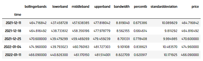
bb_dataframe = pd.DataFrame(window).set_index('time')

Jupyter Notebooks don't currently support libraries to plot historical data, but we are working on adding the functionality. Until the functionality is added, use Python to plot indicators.

Follow these steps to plot the indicator values:

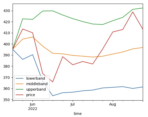
1. Select the columsn to plot.

df = bb_dataframe[['lowerband', 'middleband', 'upperband', 'price']]

2. Call the plot method.

df.plot()

3. Show the plot.

plt.show()