Applying Research
Airline Buybacks
Create Hypothesis
Buyback represents a company buy back its own stocks in the market, as (1) management is confident on its own future, and (2) wants more control over its development. Since usually buyback is in large scale on a schedule, the price of repurchasing often causes price fluctuation.
Airlines is one of the largest buyback sectors. Major US Airlines use over 90% of their free cashflow to buy back their own stocks in the recent years.[1] Therefore, we can use airline companies to test the hypothesis of buybacks would cause price action. In this particular exmaple, we're hypothesizing that difference in buyback price and close price would suggest price change in certain direction. (we don't know forward return would be in momentum or mean-reversion in this case!)
Import Libraries
We'll need to import libraries to help with data processing, validation and visualization. Import SmartInsiderTransaction class, statsmodels, sklearn, numpy, pandas and seaborn libraries by the following:
from QuantConnect.DataSource import SmartInsiderTransaction

from statsmodels.discrete.discrete_model import Logit
from sklearn.metrics import confusion_matrix
import numpy as np
import pandas as pd
import seaborn as sns
Get Historical Data
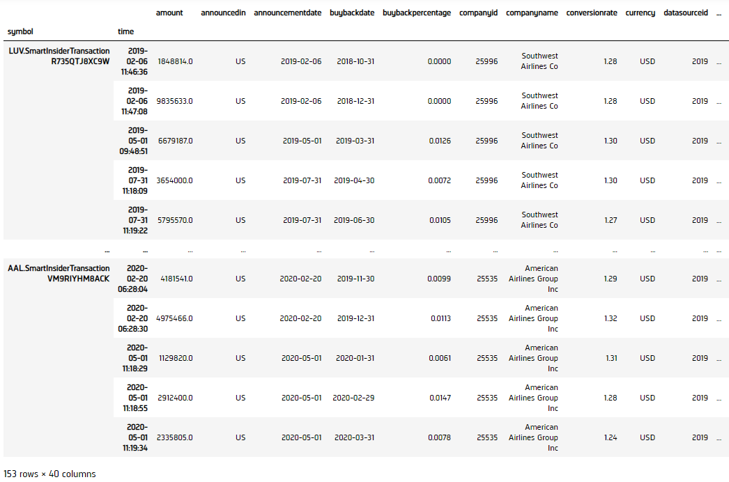
To begin, we retrieve historical data for researching.
- Instantiate a
QuantBook. - Select the airline tickers for research.
- Call the
add_equitymethod with the tickers, and its corresponding resolution. Then calladd_datawithSmartInsiderTransactionto subscribe to their buyback transaction data. Save theSymbols into a dictionary. - Call the
historymethod with a list ofSymbols for all tickers, time argument(s), and resolution to request historical data for the symbols. - Call SPY history as reference.
- Call the
historymethod with a list ofSmartInsiderTransactionSymbols for all tickers, time argument(s), and resolution to request historical data for the symbols.
qb = QuantBook()
assets = ["LUV",   # Southwest Airlines
          "DAL",   # Delta Airlines
          "UAL",   # United Airlines Holdings
          "AAL",   # American Airlines Group
          "SKYW",  # SkyWest Inc.
          "ALGT",  # Allegiant Travel Co.
          "ALK"    # Alaska Air Group Inc.
         ]
symbols = {}
for ticker in assets:
    symbol = qb.add_equity(ticker, Resolution.MINUTE).symbol
    symbols[symbol] = qb.add_data(SmartInsiderTransaction, symbol).symbol
If you do not pass a resolution argument, Resolution.MINUTE is used by default.
history = qb.history(list(symbols.keys()), datetime(2019, 1, 1), datetime(2021, 12, 31), Resolution.DAILY)
spy = qb.history(qb.add_equity("SPY").symbol, datetime(2019, 1, 1), datetime(2021, 12, 31), Resolution.DAILY)
history_buybacks = qb.history(list(symbols.values()), datetime(2019, 1, 1), datetime(2021, 12, 31), Resolution.DAILY)
Prepare Data
We'll have to process our data to get the buyback premium/discount% vs forward return data.
- Select the close column and then call the
unstackmethod. - Call
pct_changeto get the daily return of close price, then shift 1-step backward as prediction. - Get the active forward return.
- Select the ExecutionPrice column and then call the
unstackmethod to get the buyback dataframe. - Convert buyback history into daily mean data.
- Get the buyback premium/discount %.
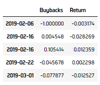
- Create a
Dataframeto hold the buyback and 1-day forward return data. - Append the data into the
Dataframe. - Call
dropnato drop NaNs.
df = history['close'].unstack(level=0)
spy_close = spy['close'].unstack(level=0)
ret = df.pct_change().shift(-1).iloc[:-1]
ret_spy = spy_close.pct_change().shift(-1).iloc[:-1]
active_ret = ret.sub(ret_spy.values, axis=0)
df_buybacks = history_buybacks['executionprice'].unstack(level=0)
df_buybacks = df_buybacks.groupby(df_buybacks.index.date).mean()
df_buybacks.columns = df.columns
df_close = df.reindex(df_buybacks.index)[~df_buybacks.isna()]
df_buybacks = (df_buybacks - df_close)/df_close
data = pd.DataFrame(columns=["Buybacks", "Return"])
for row, row_buyback in zip(active_ret.reindex(df_buybacks.index).itertuples(), df_buybacks.itertuples()):
    index = row[0]
    for i in range(1, df_buybacks.shape[1]+1):
        if row_buyback[i] != 0:
            data = pd.concat([data, pd.DataFrame({"Buybacks": row_buyback[i], "Return":row[i]}, index=[index])])
data.dropna(inplace=True)
Test Hypothesis
We would test (1) if buyback has statistically significant effect on return direction, and (2) buyback could be a return predictor.
- Get binary return (+/-).
- Construct a logistic regression model.
- Display logistic regression results.
- Plot the results.
- Get in-sample prediction result.
- Call
confusion_matrixto contrast the results. - Display the result.
binary_ret = data["Return"].copy()
binary_ret[binary_ret < 0] = 0
binary_ret[binary_ret > 0] = 1
model = Logit(binary_ret.values, data["Buybacks"].values).fit()
display(model.summary())
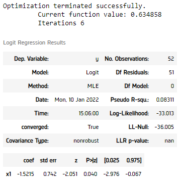
We can see a p-value of < 0.05 in the logistic regression model, meaning the separation of positive and negative using buyback premium/discount% is statistically significant.
plt.figure(figsize=(10, 6))
sns.regplot(x=data["Buybacks"]*100, y=binary_ret, logistic=True, ci=None, line_kws={'label': " Logistic Regression Line"})
plt.plot([-50, 50], [0.5, 0.5], "r--", label="Selection Cutoff Line")
plt.title("Buyback premium vs Profit/Loss")
plt.xlabel("Buyback premium %")
plt.xlim([-50, 50])
plt.ylabel("Profit/Loss")
plt.legend()
plt.show()
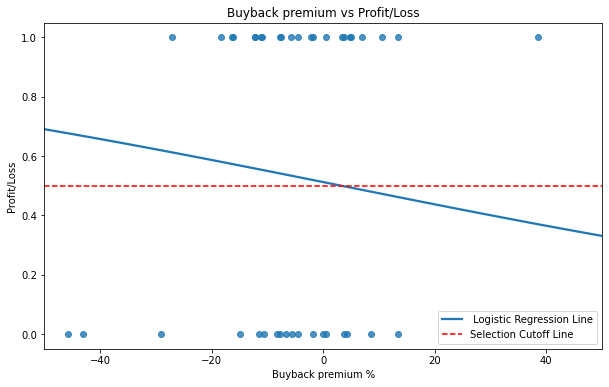
Interesting, from the logistic regression line, we observe that when the airlines brought their stock in premium price, the price tended to go down, while the opposite for buying back in discount.
Let's also study how good is the logistic regression.
predictions = model.predict(data["Buybacks"].values)
for i in range(len(predictions)):
    predictions[i] = 1 if predictions[i] > 0.5 else 0
cm = confusion_matrix(binary_ret, predictions)
df_result = pd.DataFrame(cm,
                        index=pd.MultiIndex.from_tuples([("Prediction", "Positive"), ("Prediction", "Negative")]),
                        columns=pd.MultiIndex.from_tuples([("Actual", "Positive"), ("Actual", "Negative")]))
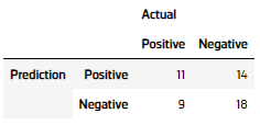
The logistic regression is having a 55.8% accuracy (55% sensitivity and 56.3% specificity), this can suggest a > 50% win rate before friction costs, proven our hypothesis.
Set Up Algorithm
Once we are confident in our hypothesis, we can export this code into backtesting. One way to accomodate this model into backtest is to create a scheduled event which uses our model to predict the expected return.
def initialize(self) -> None:

    #1. Required: Five years of backtest history
    self.set_start_date(2017, 1, 1)

    #2. Required: Alpha Streams Models:
    self.set_brokerage_model(BrokerageName.ALPHA_STREAMS)

    #3. Required: Significant AUM Capacity
    self.set_cash(1000000)

    #4. Required: Benchmark to SPY
    self.set_benchmark("SPY")

    self.set_portfolio_construction(EqualWeightingPortfolioConstructionModel())
    self.set_execution(ImmediateExecutionModel())

    # Set our strategy to be take 5% profit and 5% stop loss.
    self.add_risk_management(MaximumUnrealizedProfitPercentPerSecurity(0.05))
    self.add_risk_management(MaximumDrawdownPercentPerSecurity(0.05))

    # Select the airline tickers for research.
    self.symbols = {}
    assets = ["LUV",   # Southwest Airlines
                "DAL",   # Delta Airlines
                "UAL",   # United Airlines Holdings
                "AAL",   # American Airlines Group
                "SKYW",  # SkyWest Inc.
                "ALGT",  # Allegiant Travel Co.
                "ALK"    # Alaska Air Group Inc.
                ]

    # Call the AddEquity method with the tickers, and its corresponding resolution. Then call AddData with SmartInsiderTransaction to subscribe to their buyback transaction data.
    for ticker in assets:
        symbol = self.add_equity(ticker, Resolution.MINUTE).symbol
        self.symbols[symbol] = self.add_data(SmartInsiderTransaction, symbol).symbol

    self.add_equity("SPY")

    # Initialize the model
    self.build_model()

    # Set Scheduled Event Method For Our Model Recalibration every month
    self.schedule.on(self.date_rules.month_start(), self.time_rules.at(0, 0), self.build_model)

    # Set Scheduled Event Method For Trading
    self.schedule.on(self.date_rules.every_day(), self.time_rules.before_market_close("SPY", 5), self.every_day_before_market_close)
We'll also need to create a function to train and update the logistic regression model from time to time.
def build_model(self) -> None:
    qb = self
    # Call the History method with list of tickers, time argument(s), and resolution to request historical data for the symbol.
    history = qb.history(list(self.symbols.keys()), datetime(2015, 1, 1), datetime.now(), Resolution.DAILY)

    # Call SPY history as reference
    spy = qb.history(["SPY"], datetime(2015, 1, 1), datetime.now(), Resolution.DAILY)

    # Call the History method with list of buyback tickers, time argument(s), and resolution to request buyback data for the symbol.
    history_buybacks = qb.history(list(self.symbols.values()), datetime(2015, 1, 1), datetime.now(), Resolution.DAILY)

    # Select the close column and then call the unstack method to get the close price dataframe.
    df = history['close'].unstack(level=0)
    spy_close = spy['close'].unstack(level=0)

    # Call pct_change to get the daily return of close price, then shift 1-step backward as prediction.
    ret = df.pct_change().shift(-1).iloc[:-1]
    ret_spy = spy_close.pct_change().shift(-1).iloc[:-1]

    # Get the active return
    active_ret = ret.sub(ret_spy.values, axis=0)

    # Select the ExecutionPrice column and then call the unstack method to get the dataframe.
    df_buybacks = history_buybacks['executionprice'].unstack(level=0)

    # Convert buyback history into daily mean data
    df_buybacks = df_buybacks.groupby(df_buybacks.index.date).mean()
    df_buybacks.columns = df.columns

    # Get the buyback premium/discount
    df_close = df.reindex(df_buybacks.index)[~df_buybacks.isna()]
    df_buybacks = (df_buybacks - df_close)/df_close

    # Create a dataframe to hold the buyback and 1-day forward return data
    data = pd.DataFrame(columns=["Buybacks", "Return"])

    # Append the data into the dataframe
    for row, row_buyback in zip(active_ret.reindex(df_buybacks.index).itertuples(), df_buybacks.itertuples()):
        index = row[0]
        for i in range(1, df_buybacks.shape[1]+1):
            if row_buyback[i] != 0:
                data = pd.concat([data, pd.DataFrame({"Buybacks": row_buyback[i], "Return":row[i]}, index=[index])])

    # Call dropna to drop NaNs
    data.dropna(inplace=True)

    # Get binary return (+/-)
    binary_ret = data["Return"].copy()
    binary_ret[binary_ret < 0] = 0
    binary_ret[binary_ret > 0] = 1

    # Construct a logistic regression model
    self.model = Logit(binary_ret.values, data["Buybacks"].values).fit()
Now we export our model into the scheduled event method. We will switch qb with self and replace methods with their QCAlgorithm counterparts as needed. In this example, this is not an issue because all the methods we used in research also exist in QCAlgorithm.
def every_day_before_market_close(self) -> None:
    qb = self
    # Get any buyback event today
    history_buybacks = qb.history(list(self.symbols.values()), timedelta(days=1), Resolution.DAILY)
    if history_buybacks.empty or "executionprice" not in history_buybacks.columns: return

    # Select the ExecutionPrice column and then call the unstack method to get the dataframe.
    df_buybacks = history_buybacks['executionprice'].unstack(level=0)

    # Convert buyback history into daily mean data
    df_buybacks = df_buybacks.groupby(df_buybacks.index.date).mean()

    # ==============================

    insights = []

    # Iterate the buyback data, thne pass to the model for prediction
    row = df_buybacks.iloc[-1]
    for i in range(len(row)):
        prediction = self.model.predict(row[i])

        # Long if the prediction predict price goes up, short otherwise. Do opposite for SPY (active return)
        if prediction > 0.5:
            insights.append( Insight.price(row.index[i].split(".")[0], timedelta(days=1), InsightDirection.UP) )
            insights.append( Insight.price("SPY", timedelta(days=1), InsightDirection.DOWN) )
        else:
            insights.append( Insight.price(row.index[i].split(".")[0], timedelta(days=1), InsightDirection.DOWN) )
            insights.append( Insight.price("SPY", timedelta(days=1), InsightDirection.UP) )

    self.emit_insights(insights)
Examples
The below code snippets concludes the above jupyter research notebook content.
from QuantConnect.DataSource import SmartInsiderTransaction
from statsmodels.discrete.discrete_model import Logit
from sklearn.metrics import confusion_matrix
import seaborn as sns

# Instantiate a QuantBook.
qb = QuantBook()

# Select the airline tickers for research.
assets = ["LUV",   # Southwest Airlines
          "DAL",   # Delta Airlines
          "UAL",   # United Airlines Holdings
          "AAL",   # American Airlines Group
          "SKYW",  # SkyWest Inc.
          "ALGT",  # Allegiant Travel Co.
          "ALK"    # Alaska Air Group Inc.
         ]

# Call the AddEquity method with the tickers, and its corresponding resolution. Then call AddData with SmartInsiderTransaction to subscribe to their buyback transaction data. Save the Symbols into a dictionary.
symbols = {}
for ticker in assets:
    Symbol = qb.add_equity(ticker, Resolution.MINUTE).symbol
    symbols[Symbol] = qb.add_data(SmartInsiderTransaction, Symbol).symbol

# Call the History method with list of tickers, time argument(s), and resolution to request historical data for the symbol.
history = qb.history(list(symbols.keys()), datetime(2019, 1, 1), datetime(2021, 12, 31), Resolution.DAILY)

# Call SPY history as reference.
spy = qb.history(qb.add_equity("SPY").symbol, datetime(2019, 1, 1), datetime(2021, 12, 31), Resolution.DAILY)

# Call the History method with list of buyback tickers, time argument(s), and resolution to request buyback data for the symbol.
history_buybacks = qb.history(list(symbols.values()), datetime(2019, 1, 1), datetime(2021, 12, 31), Resolution.DAILY)

# Select the close column and then call the unstack method to get the close price dataframe.
df = history['close'].unstack(level=0)
spy_close = spy['close'].unstack(level=0)

# Call pct_change to get the daily return of close price, then shift 1-step backward as prediction.
ret = df.pct_change().shift(-1).iloc[:-1]
ret_spy = spy_close.pct_change().shift(-1).iloc[:-1]

# Get the active forward return.
active_ret = ret.sub(ret_spy.values, axis=0)

# Select the ExecutionPrice column and then call the unstack method to get the dataframe.
# Remove duplicate values from the index
history_buybacks = history_buybacks[~history_buybacks.index.duplicated(keep='first')]
df_buybacks = history_buybacks['executionprice'].unstack(level=0)

# Convert buyback history into daily mean data.
df_buybacks = df_buybacks.groupby(df_buybacks.index.date).mean()
df_buybacks.columns = df.columns

# Get the buyback premium/discount %.
df_close = df.reindex(df_buybacks.index)[~df_buybacks.isna()]
df_buybacks = (df_buybacks - df_close)/df_close

# Create a dataframe to hold the buyback and 1-day forward return data.
data = pd.DataFrame(columns=["Buybacks", "Return"])

# Append the data into the dataframe.
for row, row_buyback in zip(active_ret.reindex(df_buybacks.index).itertuples(), df_buybacks.itertuples()):
    index = row[0]
    for i in range(1, df_buybacks.shape[1]+1):
        if row_buyback[i] != 0:
            data = pd.concat([data, pd.DataFrame({"Buybacks": row_buyback[i], "Return":row[i]}, index=[index])])

# Call dropna to drop NaNs.
data.dropna(inplace=True)

# Get binary return (+/-).
binary_ret = data["Return"].copy()
binary_ret[binary_ret < 0] = 0
binary_ret[binary_ret > 0] = 1

# Construct a logistic regression model.
model = Logit(binary_ret.values, data["Buybacks"].values).fit()

# Display logistic regression results.
display(model.summary())

# Plot the result.
plt.figure(figsize=(10, 6))
sns.regplot(x=data["Buybacks"]*100, y=binary_ret, logistic=True, ci=None, line_kws={'label': " Logistic Regression Line"})
plt.plot([-50, 50], [0.5, 0.5], "r--", label="Selection Cutoff Line")
plt.title("Buyback premium vs Profit/Loss")
plt.xlabel("Buyback premium %")
plt.xlim([-50, 50])
plt.ylabel("Profit/Loss")
plt.legend()
plt.show()

# Get in-sample prediction result.
predictions = model.predict(data["Buybacks"].values)
for i in range(len(predictions)):
    predictions[i] = 1 if predictions[i] > 0.5 else 0

# Call confusion_matrix to contrast the results.
cm = confusion_matrix(binary_ret, predictions)

# Display the result.
df_result = pd.DataFrame(cm,
                        index=pd.MultiIndex.from_tuples([("Prediction", "Positive"), ("Prediction", "Negative")]),
                        columns=pd.MultiIndex.from_tuples([("Actual", "Positive"), ("Actual", "Negative")]))
The below code snippets concludes the algorithm set up.
from statsmodels.discrete.discrete_model import Logit

class AirlineBuybacksDemo(QCAlgorithm):
    def initialize(self) -> None:
        self.set_start_date(2024, 9, 1)
        self.set_end_date(2024, 12, 31)
        self.set_cash(1000000)
        self.settings.daily_precise_end_time = False
        self.set_benchmark("SPY")
        self.set_portfolio_construction(EqualWeightingPortfolioConstructionModel())
        self.set_execution(ImmediateExecutionModel())

        # Set our strategy to be take 5% profit and 5% stop loss.
        self.add_risk_management(MaximumUnrealizedProfitPercentPerSecurity(0.05))
        self.add_risk_management(MaximumDrawdownPercentPerSecurity(0.05))

        # Select the airline tickers for research.
        self.symbols = {}
        assets = ["LUV",   # Southwest Airlines
                  "DAL",   # Delta Airlines
                  "UAL",   # United Airlines Holdings
                  "AAL",   # American Airlines Group
                  "SKYW",  # SkyWest Inc.
                  "ALGT",  # Allegiant Travel Co.
                  "ALK"    # Alaska Air Group Inc.
                 ]

        # Call the AddEquity method with the tickers, and its corresponding resolution. Then call AddData with SmartInsiderTransaction to subscribe to their buyback transaction data.
        for ticker in assets:
            symbol = self.add_equity(ticker, Resolution.MINUTE).symbol
            self.symbols[symbol] = self.add_data(SmartInsiderTransaction, symbol).symbol

        self.add_equity("SPY")

        # Initialize the model
        self.build_model()

        # Set Scheduled Event Method For Our Model Recalibration every month
        self.schedule.on(self.date_rules.month_start(), self.time_rules.at(0, 0), self.build_model)

        # Set Scheduled Event Method For Trading
        self.schedule.on(self.date_rules.every_day(), self.time_rules.before_market_close("SPY", 5), self.every_day_before_market_close)


    def build_model(self) -> None:
        qb = self
        # Call the History method with list of tickers, time argument(s), and resolution to request historical data for the symbol.
        history = qb.history(list(self.symbols.keys()), datetime(2015, 1, 1), self.time, Resolution.DAILY)

        # Call SPY history as reference
        spy = qb.history(["SPY"], datetime(2015, 1, 1), self.time, Resolution.DAILY)

        # Call the History method with list of buyback tickers, time argument(s), and resolution to request buyback data for the symbol.
        history_buybacks = qb.history(list(self.symbols.values()), datetime(2015, 1, 1), self.time, Resolution.DAILY)

        # Select the close column and then call the unstack method to get the close price dataframe.
        df = history['close'].unstack(level=0)
        spy_close = spy['close'].unstack(level=0)

        # Call pct_change to get the daily return of close price, then shift 1-step backward as prediction.
        ret = df.pct_change().shift(-1).iloc[:-1]
        ret_spy = spy_close.pct_change().shift(-1).iloc[:-1]

        # Get the active return
        active_ret = ret.sub(ret_spy.values, axis=0)

        # Select the ExecutionPrice column and then call the unstack method to get the dataframe.
        history_buybacks = history_buybacks[~history_buybacks.index.duplicated(keep='first')]
        df_buybacks = history_buybacks['executionprice'].unstack(level=0)

        # Convert buyback history into daily mean data
        df_buybacks = df_buybacks.groupby(df_buybacks.index.date).mean()
        df_buybacks.columns = df.columns

        # Get the buyback premium/discount
        df_close = df.reindex(df_buybacks.index)[~df_buybacks.isna()]
        df_buybacks = (df_buybacks - df_close)/df_close

        # Create a dataframe to hold the buyback and 1-day forward return data
        data = pd.DataFrame(columns=["Buybacks", "Return"])

        # Append the data into the dataframe
        for row, row_buyback in zip(active_ret.reindex(df_buybacks.index).itertuples(), df_buybacks.itertuples()):
            index = row[0]
            for i in range(1, df_buybacks.shape[1]+1):
                if row_buyback[i] != 0:
                    data = pd.concat([data, pd.DataFrame({"Buybacks": row_buyback[i], "Return":row[i]}, index=[index])])

        # Call dropna to drop NaNs
        data.dropna(inplace=True)

        # Get binary return (+/-)
        binary_ret = data["Return"].copy()
        binary_ret[binary_ret < 0] = 0
        binary_ret[binary_ret > 0] = 1

        # Construct a logistic regression model
        self.model = Logit(binary_ret.values, data["Buybacks"].values).fit()


    def every_day_before_market_close(self) -> None:
        qb = self
        # Get any buyback event today
        history_buybacks = qb.history(list(self.symbols.values()), timedelta(days=1), Resolution.DAILY)
        if history_buybacks.empty or "executionprice" not in history_buybacks.columns: return

        # Select the ExecutionPrice column and then call the unstack method to get the dataframe.
        history_buybacks = history_buybacks[~history_buybacks.index.duplicated(keep='first')]
        df_buybacks = history_buybacks['executionprice'].unstack(level=0)

        # Convert buyback history into daily mean data
        df_buybacks = df_buybacks.groupby(df_buybacks.index.date).mean()

        # ==============================

        insights = []

        # Iterate the buyback data, thne pass to the model for prediction
        row = df_buybacks.iloc[-1]
        for i in range(len(row)):
            prediction = self.model.predict(row[i])

            # Long if the prediction predict price goes up, short otherwise. Do opposite for SPY (active return)
            if prediction > 0.5:
                insights.append( Insight.price(row.index[i].underlying, timedelta(days=1), InsightDirection.UP) )
                insights.append( Insight.price("SPY", timedelta(days=1), InsightDirection.DOWN) )
            else:
                insights.append( Insight.price(row.index[i].underlying, timedelta(days=1), InsightDirection.DOWN) )
                insights.append( Insight.price("SPY", timedelta(days=1), InsightDirection.UP) )

        self.emit_insights(insights)
You can also see our Videos. You can also get in touch with us via Discord.
Did you find this page helpful?