Meta Analysis
Live Reconciliation
Introduction
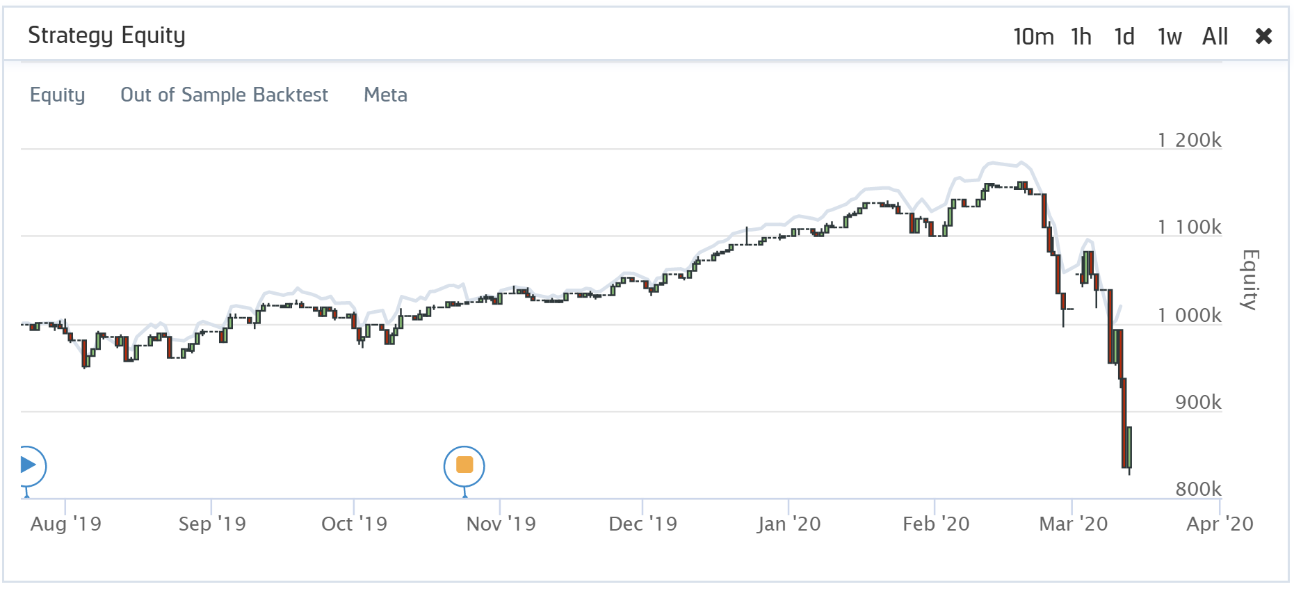
This page shows you how to generate the out-of-sample (OOS) backtest reconciliation curve from a live deployment in the Research Environment so you can quantitatively and visually compare live versus backtest performance. You read the live deployment's launch datetime and starting equity, run a backtest with matching parameters, and overlay the two "Strategy Equity" curves along with every order fill on a single chart per security.
Reconciliation is a way to quantify the difference between an algorithm's live performance and its out-of-sample (OOS) performance (a backtest run over the live deployment period).
Seeing the difference between live performance and OOS performance gives you a way to determine if the algorithm is making unrealistic assumptions, exploiting data differences, or merely exhibiting behavior that is impractical or impossible in live trading.
A perfectly reconciled algorithm has an exact overlap between its live equity and OOS backtest curves. Any deviation means that the performance of the algorithm has differed for some reason. Several factors can contribute to this, often stemming from the algorithm design. For a catalogue of common deviation causes (data, modeling, brokerage, third-party indicators, and real-time scheduled events), see Reconciliation in the Writing Algorithms documentation.
Reconciliation is scored using two metrics: returns correlation and dynamic time warping (DTW) distance.
What is DTW Distance?
Dynamic Time Warp (DTW) Distance quantifies the difference between two time-series. It is an algorithm that measures the shortest path between the points of two time-series. It uses Euclidean distance as a measurement of point-to-point distance and returns an overall measurement of the distance on the scale of the initial time-series values. We apply DTW to the returns curve of the live and OOS performance, so the DTW distance measurement is on the scale of percent returns.
$$\begin{equation} DTW(X,Y) = min\bigg\{\sum_{l=1}^{L}\left(x_{m_l} - y_{n_l}\right)^{2}\in P^{N\times M}\bigg\} \end{equation}$$For the reasons outlined in our research notebook on the topic (linked below), QuantConnect annualizes the daily DTW. An annualized distance provides a user with a measurement of the annual difference in the magnitude of returns between the two curves. A perfect score is 0, meaning the returns for each day were precisely the same. A DTW score of 0 is nearly impossible to achieve, and we consider anything below 0.2 to be a decent score. A distance of 0.2 means the returns between an algorithm's live and OOS performance deviated by 20% over a year.
What is Returns Correlation?
Returns correlation is the simple Pearson correlation between the live and OOS returns. Correlation gives us a rudimentary understanding of how the returns move together. Do they trend up and down at the same time? Do they deviate in direction or timing?
$$\begin{equation} \rho_{XY} = \frac{cov(X, Y)}{\sigma_X\sigma_Y} \end{equation}$$An algorithm's returns correlation should be as close to 1 as possible. We consider a good score to be 0.8 or above, meaning that there is a strong positive correlation. This indicates that the returns move together most of the time and that for any given return you see from one of the curves, the other curve usually has a similar direction return (positive or negative).
Why Do We Need Both DTW and Returns Correlation?
Each measurement provides insight into distinct elements of time-series similarity, but neither measurement alone gives us the whole picture. Returns correlation tells us whether or not the live and OOS returns move together, but it doesn't account for the possible differences in the magnitude of the returns. DTW distance measures the difference in magnitude of returns but provides no insight into whether or not the returns move in the same direction. It is possible for there to be two cases of equity curve similarity where both pairs have the same DTW distance, but one has perfectly negatively correlated returns, and the other has a perfectly positive correlation. Similarly, it is possible for two pairs of equity curves to each have perfect correlation but substantially different DTW distance. Having both measurements provides us with a more comprehensive understanding of the actual similarity between live and OOS performance. We outline several interesting cases and go into more depth on the topic of reconciliation in research we have published.
Get Live Deployment Parameters
Follow these steps to read the live deployment's start datetime, starting equity, and end datetime — the three parameters the OOS backtest must match. All three values come from the live "Strategy Equity" chart, so you only need the project Id.
- Define the project Id.
- Read the live "Strategy Equity" chart with the
ReadLiveChartread_live_chartmethod. The first and lastEquitypoints give you the start datetime, starting equity, and end datetime.
var projectId = 23034953;
project_id = 23034953
The following table provides links to documentation that explains how to get the project Id, depending on the platform you use:
| Platform | Project Id |
|---|---|
| Cloud Platform | Get Project Id |
| Local Platform | Get Project Id |
| CLI | Get Project Id |
var nowSec = (int)DateTimeOffset.UtcNow.ToUnixTimeSeconds();

Chart ReadLiveChartWithRetry(int projectId, string chartName)
{
    for (var attempt = 0; attempt < 10; attempt++)
    {
        var result = api.ReadLiveChart(projectId, chartName, 0, nowSec, 500);
        if (result.Success) return result.Chart;
        Console.WriteLine($"Chart data is loading... (attempt {attempt + 1}/10)");
        Thread.Sleep(10000);
    }
    throw new Exception($"Failed to read {chartName} chart after 10 attempts");
}

var strategyEquity = ReadLiveChartWithRetry(projectId, "Strategy Equity");
// The first few points in the series can have a null close, so keep only
// the points with a valid close value before extracting start/end.
var validValues = strategyEquity.Series["Equity"].Values
    .OfType<Candlestick>()
    .Where(v => v.Close.HasValue)
    .ToList();

// Start datetime and starting equity: first valid point.
var startDatetime = validValues.First().Time;
var startingCash = validValues.First().Close.Value;
// End datetime: last valid timestamp of the live Strategy Equity series.
// Uncomment the next line instead to reconcile up to "now" and see what
// would have happened had you not stopped the live algorithm:
// var endDatetime = DateTime.UtcNow;
var endDatetime = validValues.Last().Time;

Console.WriteLine($"Start (UTC): {startDatetime}");
Console.WriteLine($"Starting equity: ${startingCash:N2}");
Console.WriteLine($"End (UTC): {endDatetime}");
from datetime import datetime
from time import sleep, time
def read_chart(project_id, chart_name, start=0, end=int(time()), count=500):
# Retry up to 10 times until the chart data finishes loading.
for attempt in range(10):
result = api.read_live_chart(project_id, chart_name, start, end, count)
if result.success:
return result.chart
print(f"Chart data is loading... (attempt {attempt + 1}/10)")
sleep(10)
raise RuntimeError(f"Failed to read {chart_name} chart after 10 attempts")
strategy_equity = read_chart(project_id, 'Strategy Equity')
# The first few points in the series can have a None close, so keep only
# the points with a valid close value before extracting start/end.
valid_values = [v for v in strategy_equity.series['Equity'].values if v.close is not None]
# Start datetime and starting equity: first valid point.
start_datetime = valid_values[0].time
starting_cash = valid_values[0].close
# End datetime: last valid timestamp of the live Strategy Equity series.
# Uncomment the next line instead to reconcile up to "now" and see what
# would have happened had you not stopped the live algorithm:
# end_datetime = datetime.utcnow()
end_datetime = valid_values[-1].time
print(f"Start (UTC): {start_datetime}")
print(f"Starting equity: ${starting_cash:,.2f}")
print(f"End (UTC): {end_datetime}")
Run OOS Backtest
Follow these steps to run an out-of-sample backtest that mirrors the live deployment.
- In the project's main algorithm file, set the start date and starting cash to match the values you read in the previous step. Use
SetStartDateset_start_dateandSetCashset_cashso the backtest begins at the same moment and with the same equity as the live deployment. You can either hard-code the values or expose them as parameters. - Compile the project by calling the
CreateCompilecreate_compilemethod, then pollReadCompileread_compileuntil the compile state isBuildSuccess. - Create the OOS backtest with the
CreateBacktestcreate_backtestmethod. - Poll the
ReadBacktestread_backtestmethod until thecompletedflag isTrue. Log theprogressattribute on each poll so you can watch the backtest advance.
var compilation = api.CreateCompile(projectId);
var compileId = compilation.CompileId;

// Poll until the build succeeds.
for (var attempt = 0; attempt < 10; attempt++)
{
    var result = api.ReadCompile(projectId, compileId);
    if (result.State == CompileState.BuildSuccess) break;
    if (result.State == CompileState.BuildError)
    {
        throw new Exception($"Compilation failed: {string.Join(Environment.NewLine, result.Logs)}");
    }
    Console.WriteLine($"Compile in queue... (attempt {attempt + 1}/10)");
    Thread.Sleep(5000);
}
from time import sleep
compilation = api.create_compile(project_id)
compile_id = compilation.compile_id
# Poll until the build succeeds.
for attempt in range(10):
result = api.read_compile(project_id, compile_id)
if result.state == 'BuildSuccess':
break
if result.state == 'BuildError':
raise Exception(f"Compilation failed: {result.logs}")
print(f"Compile in queue... (attempt {attempt + 1}/10)")
sleep(5)
var backtest = api.CreateBacktest(projectId, compileId, "OOS Reconciliation");
var backtestId = backtest.BacktestId;
Console.WriteLine($"Backtest Id: {backtestId}");
backtest = api.create_backtest(project_id, compile_id, 'OOS Reconciliation')
backtest_id = backtest.backtest_id
print(f"Backtest Id: {backtest_id}")
var completed = false;
while (!completed)
{
    var result = api.ReadBacktest(projectId, backtestId);
    completed = result.Completed;
    Console.WriteLine($"Backtest running... {result.Progress:P2}");
    Thread.Sleep(10000);
}
Console.WriteLine("Backtest completed.");
completed = False
while not completed:
result = api.read_backtest(project_id, backtest_id)
completed = result.completed
print(f"Backtest running... {result.progress:.2%}")
sleep(10)
print("Backtest completed.")
Plot Equity Curves
Follow these steps to plot the live and OOS backtest equity curves on the same axes.
- Read the live "Strategy Equity" chart using the retry helper from the previous step.
- Read the backtest "Strategy Equity" chart by calling the
ReadBacktestChartread_backtest_chartmethod with the same retry pattern. - Extract the
Equityseries from each chart, filtering out points with a null close. Python uses apandas.Seriesindexed by timestamp so the two curves can be aligned on the union of their timestamps; C# keeps two lists ofCandlestickpoints and lets Plotly.NET align them on the same x-axis. - Plot both curves on the same axis. Python uses
matplotlib; C# uses Plotly.NET — loadPlotly.NETandPlotly.NET.Interactivefrom NuGet and aliasPlotly.NET.Chartto avoid ambiguity withQuantConnect.Chart. - Score the reconciliation with the annualized returns DTW distance and the Pearson correlation of daily returns. Use
tslearn'sdtwwith a Sakoe-Chiba band so the algorithm runs in linear time. Thetslearnlibrary is Python-only; run this step in a Python research notebook.
var liveEquityChart = ReadLiveChartWithRetry(projectId, "Strategy Equity");
live_equity_chart = read_chart(project_id, 'Strategy Equity')
Chart ReadBacktestChartWithRetry(int projectId, string backtestId, string chartName)
{
    for (var attempt = 0; attempt < 10; attempt++)
    {
        var result = api.ReadBacktestChart(projectId, chartName, 0, nowSec, 500, backtestId);
        if (result.Success) return result.Chart;
        Console.WriteLine($"Chart data is loading... (attempt {attempt + 1}/10)");
        Thread.Sleep(10000);
    }
    throw new Exception($"Failed to read backtest {chartName} chart after 10 attempts");
}

var backtestEquityChart = ReadBacktestChartWithRetry(projectId, backtestId, "Strategy Equity");
def read_backtest_chart(project_id, backtest_id, chart_name, start=0, end=int(time()), count=500):
for attempt in range(10):
result = api.read_backtest_chart(project_id, chart_name, start, end, count, backtest_id)
if result.success:
return result.chart
print(f"Chart data is loading... (attempt {attempt + 1}/10)")
sleep(10)
raise RuntimeError(f"Failed to read backtest {chart_name} chart after 10 attempts")
backtest_equity_chart = read_backtest_chart(project_id, backtest_id, 'Strategy Equity')
var liveValues = liveEquityChart.Series["Equity"].Values
    .OfType<Candlestick>()
    .Where(v => v.Close.HasValue)
    .ToList();
var backtestValues = backtestEquityChart.Series["Equity"].Values
    .OfType<Candlestick>()
    .Where(v => v.Close.HasValue)
    .ToList();
import pandas as pd
def to_naive(t):
ts = pd.Timestamp(t)
return ts.tz_convert('UTC').tz_localize(None) if ts.tzinfo else ts
def to_series(chart, series_name='Equity'):
values = [v for v in chart.series[series_name].values if v.close is not None]
return pd.Series(
[v.close for v in values],
index=pd.DatetimeIndex([to_naive(v.time) for v in values])
)
live_series = to_series(live_equity_chart)
backtest_series = to_series(backtest_equity_chart)
# Keep every timestamp from both sources; align and forward-fill on the union.
df = pd.concat([live_series.rename('Live'), backtest_series.rename('OOS Backtest')], axis=1).sort_index().ffill()
#r "nuget: Plotly.NET"
#r "nuget: Plotly.NET.Interactive"
using PlotlyChart = Plotly.NET.Chart;
using Plotly.NET;
using Plotly.NET.Interactive;
using Plotly.NET.LayoutObjects;

var equityChart = PlotlyChart.Combine(new[]
{
    Chart2D.Chart.Line<DateTime, decimal, string>(
        liveValues.Select(v => v.Time),
        liveValues.Select(v => v.Close.Value),
        Name: "Live"),
    Chart2D.Chart.Line<DateTime, decimal, string>(
        backtestValues.Select(v => v.Time),
        backtestValues.Select(v => v.Close.Value),
        Name: "OOS Backtest")
}).WithTitle("Live vs OOS Backtest Equity");

display(equityChart);
import matplotlib.pyplot as plt
fig, ax = plt.subplots(figsize=(12, 6))
ax.plot(df.index, df['Live'], label='Live')
ax.plot(df.index, df['OOS Backtest'], label='OOS Backtest')
ax.set_title('Live vs OOS Backtest Equity')
ax.set_xlabel('Time')
ax.set_ylabel('Portfolio Value ($)')
ax.legend()
plt.show()
from tslearn.metrics import dtw as DynamicTimeWarping

returns = df.pct_change().dropna()

# Pearson correlation between live and OOS backtest daily returns (closer to 1 is better).
returns_correlation = returns.corr().iloc[0, 1]

# Raw DTW distance on the returns curves.
raw_dtw = DynamicTimeWarping(
    returns['Live'], returns['OOS Backtest'],
    global_constraint='sakoe_chiba', sakoe_chiba_radius=3
)
# Annualize so the distance is on the scale of yearly percent returns (closer to 0 is better).
annualized_dtw = abs(((1 + (raw_dtw / returns.shape[0])) ** 252) - 1)

print(f"Returns correlation: {returns_correlation:.3f}")
print(f"Annualized returns DTW: {annualized_dtw:.3f}")
Plot Order Fills
Follow these steps to overlay live and OOS backtest order fills on a single marker-only chart per symbol. The chart deliberately omits candlesticks and any price history so the comparison between live and backtest executions is not drowned out by other series.
- Read the live and backtest orders. Each call to
ReadLiveOrdersread_live_ordersandReadBacktestOrdersread_backtest_ordersreturns at most 100 orders, so paginate in 100-Id windows until the endpoint returns an empty window. The first window can take a few seconds to load, so retry while it is empty. - Organize the trade times and prices for each security into a dictionary for both the live and backtest fills.
- Plot one figure per symbol with four marker traces: live buys, live sells, backtest buys, backtest sells. Distinct markers keep live versus backtest executions visually separable.
List<ApiOrderResponse> ReadAllOrders(Func<int, int, List<ApiOrderResponse>> fetchWindow)
{
    var all = new List<ApiOrderResponse>();
    // Retry the first window while the response is empty (may be loading).
    List<ApiOrderResponse> first = null;
    for (var attempt = 0; attempt < 10; attempt++)
    {
        first = fetchWindow(0, 100);
        if (first.Any()) break;
        Console.WriteLine($"Orders loading... (attempt {attempt + 1}/10)");
        Thread.Sleep(10000);
    }
    if (first == null || !first.Any()) return all;
    all.AddRange(first);
    // Paginate in 100-Id windows until the endpoint returns an empty window.
    var start = 100;
    while (true)
    {
        var window = fetchWindow(start, start + 100);
        if (!window.Any()) break;
        all.AddRange(window);
        start += 100;
    }
    return all;
}

var liveOrders = ReadAllOrders((s, e) => api.ReadLiveOrders(projectId, s, e));
var backtestOrders = ReadAllOrders((s, e) => api.ReadBacktestOrders(projectId, backtestId, s, e));
Console.WriteLine($"Live orders: {liveOrders.Count}, OOS orders: {backtestOrders.Count}");
from time import sleep
def read_all_orders(fetch_window):
orders = []
# Retry the first window while the response is empty (may be loading).
first = []
for attempt in range(10):
first = fetch_window(0, 100)
if first:
break
print(f"Orders loading... (attempt {attempt + 1}/10)")
sleep(10)
if not first:
return orders
orders.extend(first)
# Paginate in 100-Id windows until the endpoint returns an empty window.
start = 100
while True:
window = fetch_window(start, start + 100)
if not window:
break
orders.extend(window)
start += 100
return orders
live_orders = read_all_orders(lambda s, e: api.read_live_orders(project_id, s, e))
backtest_orders = read_all_orders(lambda s, e: api.read_backtest_orders(project_id, backtest_id, s, e))
print(f"Live orders: {len(live_orders)}, OOS orders: {len(backtest_orders)}")
For more on the order objects returned, see Plot Order Fills in the Live Analysis documentation.
var liveBySymbol = liveOrders.Select(x => x.Order).GroupBy(o => o.Symbol);
var backtestBySymbol = backtestOrders.Select(x => x.Order)
    .GroupBy(o => o.Symbol)
    .ToDictionary(g => g.Key, g => g.ToList());
import pandas as pd
def to_naive(t):
# Strip tzinfo so plotly can serialize the fill times.
ts = pd.Timestamp(t)
return ts.tz_convert('UTC').tz_localize(None) if ts.tzinfo else ts
class OrderData:
def __init__(self):
self.buy_fill_times = []
self.buy_fill_prices = []
self.sell_fill_times = []
self.sell_fill_prices = []
def group_by_symbol(orders):
data_by_symbol = {}
for order in [x.order for x in orders]:
if order.symbol not in data_by_symbol:
data_by_symbol[order.symbol] = OrderData()
data = data_by_symbol[order.symbol]
is_buy = order.quantity > 0
(data.buy_fill_times if is_buy else data.sell_fill_times).append(to_naive(order.last_fill_time))
(data.buy_fill_prices if is_buy else data.sell_fill_prices).append(order.price)
return data_by_symbol
live_by_symbol = group_by_symbol(live_orders)
backtest_by_symbol = group_by_symbol(backtest_orders)
foreach (var liveGroup in liveBySymbol)
{
    var symbol = liveGroup.Key;
    var live = liveGroup.ToList();
    var bt = backtestBySymbol.TryGetValue(symbol, out var btList) ? btList : new List<Order>();

    var traces = new[]
    {
        Chart2D.Chart.Point<DateTime, decimal, string>(
            live.Where(o => o.Quantity > 0).Select(o => o.LastFillTime ?? o.Time),
            live.Where(o => o.Quantity > 0).Select(o => o.Price),
            Name: "Live Buys"),
        Chart2D.Chart.Point<DateTime, decimal, string>(
            live.Where(o => o.Quantity < 0).Select(o => o.LastFillTime ?? o.Time),
            live.Where(o => o.Quantity < 0).Select(o => o.Price),
            Name: "Live Sells"),
        Chart2D.Chart.Point<DateTime, decimal, string>(
            bt.Where(o => o.Quantity > 0).Select(o => o.LastFillTime ?? o.Time),
            bt.Where(o => o.Quantity > 0).Select(o => o.Price),
            Name: "OOS Backtest Buys"),
        Chart2D.Chart.Point<DateTime, decimal, string>(
            bt.Where(o => o.Quantity < 0).Select(o => o.LastFillTime ?? o.Time),
            bt.Where(o => o.Quantity < 0).Select(o => o.Price),
            Name: "OOS Backtest Sells")
    };
    var fillsChart = PlotlyChart.Combine(traces).WithTitle($"{symbol} Live vs OOS Backtest Fills");
    display(fillsChart);
}
import plotly.graph_objects as go
symbols = set(live_by_symbol.keys()) | set(backtest_by_symbol.keys())
for symbol in symbols:
live = live_by_symbol.get(symbol, OrderData())
bt = backtest_by_symbol.get(symbol, OrderData())
fig = go.Figure(layout=go.Layout(
title=go.layout.Title(text=f'{symbol.value} Live vs OOS Backtest Fills'),
xaxis_title='Fill Time',
yaxis_title='Fill Price',
height=600
))
fig.add_trace(go.Scatter(
x=live.buy_fill_times, y=live.buy_fill_prices, mode='markers', name='Live Buys',
marker=go.scatter.Marker(color='aqua', symbol='triangle-up', size=12)
))
fig.add_trace(go.Scatter(
x=live.sell_fill_times, y=live.sell_fill_prices, mode='markers', name='Live Sells',
marker=go.scatter.Marker(color='indigo', symbol='triangle-down', size=12)
))
fig.add_trace(go.Scatter(
x=bt.buy_fill_times, y=bt.buy_fill_prices, mode='markers', name='OOS Backtest Buys',
marker=go.scatter.Marker(color='aqua', symbol='triangle-up-open', size=12, line=dict(width=2))
))
fig.add_trace(go.Scatter(
x=bt.sell_fill_times, y=bt.sell_fill_prices, mode='markers', name='OOS Backtest Sells',
marker=go.scatter.Marker(color='indigo', symbol='triangle-down-open', size=12, line=dict(width=2))
))
fig.show()
Note: the preceding plots only show the last fill of each trade. If your trade has partial fills, the plots only display the last fill.
Examples
Example 1: Generate an OOS Reconciliation Curve
The following example reads the live deployment's "Strategy Equity" chart, runs an OOS backtest that matches its start datetime and starting cash, and plots both the equity curves and the order fills side by side. Before running it, make sure your project's main algorithm file sets StartDatestart_date and Cashcash to match the live deployment (or reads them as parameters).
// Load the necessary assemblies.
#load "../Initialize.csx"
#load "../QuantConnect.csx"
#r "nuget: Plotly.NET"
#r "nuget: Plotly.NET.Interactive"

using QuantConnect;
using QuantConnect.Api;
using QuantConnect.Research;
using System;
using System.Linq;
using System.Threading;
using PlotlyChart = Plotly.NET.Chart;
using Plotly.NET;
using Plotly.NET.Interactive;
using Plotly.NET.LayoutObjects;

// Instantiate QuantBook instance for researching.
var qb = new QuantBook();
var projectId = qb.ProjectId;   // Replace if the live algorithm is not in this project.
var nowSec = (int)DateTimeOffset.UtcNow.ToUnixTimeSeconds();

// Read the live Strategy Equity chart. The first and last valid points give
// you the start datetime, starting cash, and end datetime.
var liveEquity = api.ReadLiveChart(projectId, "Strategy Equity", 0, nowSec, 500).Chart;
var equityValues = liveEquity.Series["Equity"].Values
    .OfType<Candlestick>()
    .Where(v => v.Close.HasValue)
    .ToList();
var startDate = equityValues.First().Time;
var startingCash = equityValues.First().Close.Value;
// Uncomment to reconcile up to "now" instead:
// var endDate = DateTime.UtcNow;
var endDate = equityValues.Last().Time;

// Compile and create the OOS backtest (start date and cash must be set in the algorithm itself).
var compilation = api.CreateCompile(projectId);
var compileId = compilation.CompileId;
while (api.ReadCompile(projectId, compileId).State != CompileState.BuildSuccess)
{
    Thread.Sleep(5000);
}
var backtest = api.CreateBacktest(projectId, compileId, "OOS Reconciliation");
var backtestId = backtest.BacktestId;

var completed = false;
while (!completed)
{
    var result = api.ReadBacktest(projectId, backtestId);
    completed = result.Completed;
    Console.WriteLine($"Backtest running... {result.Progress:P2}");
    Thread.Sleep(10000);
}
Console.WriteLine("Backtest completed.");

// Read the backtest Strategy Equity chart.
var backtestEquity = api.ReadBacktestChart(projectId, "Strategy Equity", 0, nowSec, 500, backtestId).Chart;

// Read live and backtest orders for the fill overlay. Each call returns at
// most 100 orders, so paginate in 100-Id windows until we get an empty window.
// The first window can take a few seconds to load, so retry while empty.
List<ApiOrderResponse> ReadAllOrders(Func<int, int, List<ApiOrderResponse>> fetchWindow)
{
    var all = new List<ApiOrderResponse>();
    List<ApiOrderResponse> first = null;
    for (var attempt = 0; attempt < 10; attempt++)
    {
        first = fetchWindow(0, 100);
        if (first.Any()) break;
        Thread.Sleep(10000);
    }
    if (first == null || !first.Any()) return all;
    all.AddRange(first);
    var start = 100;
    while (true)
    {
        var window = fetchWindow(start, start + 100);
        if (!window.Any()) break;
        all.AddRange(window);
        start += 100;
    }
    return all;
}

var liveOrders = ReadAllOrders((s, e) => api.ReadLiveOrders(projectId, s, e));
var backtestOrders = ReadAllOrders((s, e) => api.ReadBacktestOrders(projectId, backtestId, s, e));

Console.WriteLine($"Start: {startDate}, Starting cash: {startingCash}, End: {endDate}");
Console.WriteLine($"Live orders: {liveOrders.Count}, OOS orders: {backtestOrders.Count}");

// Overlay the two equity curves with Plotly.NET.
var backtestValues = backtestEquity.Series["Equity"].Values
    .OfType<Candlestick>()
    .Where(v => v.Close.HasValue)
    .ToList();

var equityChart = PlotlyChart.Combine(new[]
{
    Chart2D.Chart.Line<DateTime, decimal, string>(
        equityValues.Select(v => v.Time),
        equityValues.Select(v => v.Close.Value),
        Name: "Live"),
    Chart2D.Chart.Line<DateTime, decimal, string>(
        backtestValues.Select(v => v.Time),
        backtestValues.Select(v => v.Close.Value),
        Name: "OOS Backtest")
}).WithTitle("Live vs OOS Backtest Equity");
display(equityChart);

// Overlay the live and backtest fills per symbol.
var liveBySymbol = liveOrders.Select(x => x.Order).GroupBy(o => o.Symbol);
var backtestBySymbol = backtestOrders.Select(x => x.Order).GroupBy(o => o.Symbol).ToDictionary(g => g.Key, g => g.ToList());

foreach (var liveGroup in liveBySymbol)
{
    var symbol = liveGroup.Key;
    var live = liveGroup.ToList();
    var bt = backtestBySymbol.TryGetValue(symbol, out var btList) ? btList : new List<Order>();

    var traces = new[]
    {
        Chart2D.Chart.Point<DateTime, decimal, string>(
            live.Where(o => o.Quantity > 0).Select(o => o.LastFillTime ?? o.Time),
            live.Where(o => o.Quantity > 0).Select(o => o.Price),
            Name: "Live Buys"),
        Chart2D.Chart.Point<DateTime, decimal, string>(
            live.Where(o => o.Quantity < 0).Select(o => o.LastFillTime ?? o.Time),
            live.Where(o => o.Quantity < 0).Select(o => o.Price),
            Name: "Live Sells"),
        Chart2D.Chart.Point<DateTime, decimal, string>(
            bt.Where(o => o.Quantity > 0).Select(o => o.LastFillTime ?? o.Time),
            bt.Where(o => o.Quantity > 0).Select(o => o.Price),
            Name: "OOS Backtest Buys"),
        Chart2D.Chart.Point<DateTime, decimal, string>(
            bt.Where(o => o.Quantity < 0).Select(o => o.LastFillTime ?? o.Time),
            bt.Where(o => o.Quantity < 0).Select(o => o.Price),
            Name: "OOS Backtest Sells")
    };
    var fillsChart = PlotlyChart.Combine(traces).WithTitle($"{symbol} Live vs OOS Backtest Fills");
    display(fillsChart);
}
# Instantiate QuantBook instance for researching.
from datetime import datetime
from time import sleep, time
import pandas as pd
import matplotlib.pyplot as plt
import plotly.graph_objects as go
from tslearn.metrics import dtw as DynamicTimeWarping
qb = QuantBook()
project_id = qb.project_id # Replace if the live algorithm is not in this project.
# Read the live Strategy Equity chart. The first and last points give you the
# start datetime, starting cash, and end datetime.
def read_chart(project_id, chart_name, start=0, end=int(time()), count=500):
for attempt in range(10):
result = api.read_live_chart(project_id, chart_name, start, end, count)
if result.success:
return result.chart
sleep(10)
raise RuntimeError(f"Failed to read {chart_name} chart after 10 attempts")
live_equity_chart = read_chart(project_id, 'Strategy Equity')
# Skip leading points with a None close (common at the start of a deployment).
valid_values = [v for v in live_equity_chart.series['Equity'].values if v.close is not None]
start_datetime = valid_values[0].time
starting_cash = valid_values[0].close
# Uncomment to reconcile up to "now" instead:
# end_datetime = datetime.utcnow()
end_datetime = valid_values[-1].time
# Compile and create the OOS backtest (start date and cash must be set in the algorithm itself).
compilation = api.create_compile(project_id)
compile_id = compilation.compile_id
while api.read_compile(project_id, compile_id).state != 'BuildSuccess':
sleep(5)
backtest = api.create_backtest(project_id, compile_id, 'OOS Reconciliation')
backtest_id = backtest.backtest_id
completed = False
while not completed:
result = api.read_backtest(project_id, backtest_id)
completed = result.completed
print(f'Backtest running... {result.progress:.2%}')
sleep(10)
# Read the backtest Strategy Equity chart.
def read_backtest_chart(project_id, backtest_id, chart_name, start=0, end=int(time()), count=500):
for attempt in range(10):
result = api.read_backtest_chart(project_id, chart_name, start, end, count, backtest_id)
if result.success:
return result.chart
sleep(10)
raise RuntimeError(f"Failed to read backtest {chart_name} chart after 10 attempts")
backtest_equity_chart = read_backtest_chart(project_id, backtest_id, 'Strategy Equity')
# Overlay the two equity curves.
def to_naive(t):
ts = pd.Timestamp(t)
return ts.tz_convert('UTC').tz_localize(None) if ts.tzinfo else ts
def to_series(chart, series_name='Equity'):
values = [v for v in chart.series[series_name].values if v.close is not None]
return pd.Series(
[v.close for v in values],
index=pd.DatetimeIndex([to_naive(v.time) for v in values])
)
df = pd.concat([
to_series(live_equity_chart).rename('Live'),
to_series(backtest_equity_chart).rename('OOS Backtest')
], axis=1).sort_index().ffill()
fig, ax = plt.subplots(figsize=(12, 6))
ax.plot(df.index, df['Live'], label='Live')
ax.plot(df.index, df['OOS Backtest'], label='OOS Backtest')
ax.set_title('Live vs OOS Backtest Equity')
ax.set_xlabel('Time'); ax.set_ylabel('Portfolio Value ($)')
ax.legend(); plt.show()
# Score the reconciliation: returns correlation and annualized returns DTW distance.
returns = df.pct_change().dropna()
returns_correlation = returns.corr().iloc[0, 1]
raw_dtw = DynamicTimeWarping(
returns['Live'], returns['OOS Backtest'],
global_constraint='sakoe_chiba', sakoe_chiba_radius=3
)
annualized_dtw = abs(((1 + (raw_dtw / returns.shape[0])) ** 252) - 1)
print(f"Returns correlation: {returns_correlation:.3f}")
print(f"Annualized returns DTW: {annualized_dtw:.3f}")
# Overlay the live and backtest fills per symbol.
class OrderData:
def __init__(self):
self.buy_fill_times, self.buy_fill_prices = [], []
self.sell_fill_times, self.sell_fill_prices = [], []
def group_by_symbol(orders):
out = {}
for order in [x.order for x in orders]:
out.setdefault(order.symbol, OrderData())
d = out[order.symbol]
is_buy = order.quantity > 0
(d.buy_fill_times if is_buy else d.sell_fill_times).append(to_naive(order.last_fill_time))
(d.buy_fill_prices if is_buy else d.sell_fill_prices).append(order.price)
return out
def read_all_orders(fetch_window):
orders = []
first = []
for attempt in range(10):
first = fetch_window(0, 100)
if first:
break
sleep(10)
if not first:
return orders
orders.extend(first)
start = 100
while True:
window = fetch_window(start, start + 100)
if not window:
break
orders.extend(window)
start += 100
return orders
live_by_symbol = group_by_symbol(read_all_orders(lambda s, e: api.read_live_orders(project_id, s, e)))
backtest_by_symbol = group_by_symbol(read_all_orders(lambda s, e: api.read_backtest_orders(project_id, backtest_id, s, e)))
for symbol in set(live_by_symbol) | set(backtest_by_symbol):
live = live_by_symbol.get(symbol, OrderData())
bt = backtest_by_symbol.get(symbol, OrderData())
fig = go.Figure(layout=go.Layout(
title=go.layout.Title(text=f'{symbol.value} Live vs OOS Backtest Fills'),
xaxis_title='Fill Time', yaxis_title='Fill Price', height=600))
fig.add_trace(go.Scatter(x=live.buy_fill_times, y=live.buy_fill_prices, mode='markers',
name='Live Buys', marker=go.scatter.Marker(color='aqua', symbol='triangle-up', size=12)))
fig.add_trace(go.Scatter(x=live.sell_fill_times, y=live.sell_fill_prices, mode='markers',
name='Live Sells', marker=go.scatter.Marker(color='indigo', symbol='triangle-down', size=12)))
fig.add_trace(go.Scatter(x=bt.buy_fill_times, y=bt.buy_fill_prices, mode='markers',
name='OOS Backtest Buys', marker=go.scatter.Marker(color='aqua', symbol='triangle-up-open', size=12, line=dict(width=2))))
fig.add_trace(go.Scatter(x=bt.sell_fill_times, y=bt.sell_fill_prices, mode='markers',
name='OOS Backtest Sells', marker=go.scatter.Marker(color='indigo', symbol='triangle-down-open', size=12, line=dict(width=2))))
fig.show()
You can also see our Videos. You can also get in touch with us via Discord.
Did you find this page helpful?